Two studies can use the same physiological recordings, select different features, and still be learning much the same thing. The feature names disagree; the information behind them may not.
That was the problem we explored in this paper. Using heat-pain recordings, we asked which measurements helped distinguish stimulus levels, how reliably those measurements were selected, and what their relationships could tell us about the signals themselves.
The question
Imagine describing muscle activity with its root mean square, standard deviation, and average absolute amplitude. Each can be useful, but all three may largely answer the same question: how large is the signal? Adding another amplitude measure may contribute less than adding a feature that captures a change from baseline.
Pain-recognition studies had proposed different combinations of sensors and features. Simply adopting the winning list from one experiment risked overlooking useful alternatives. We wanted to distinguish disagreement about feature names from disagreement about the kinds of information needed for the task.
The study at a glance
We analyzed the existing BioVid heat-pain dataset. Participants received individually calibrated heat stimuli: a 32 °C baseline (B), the onset of pain (T1), the highest tolerable level (T4), and two intermediate temperatures (T2 and T3). These labels describe the experimental conditions, rather than a universal numerical scale of pain.
- 85
- participants
- 155
- candidate features
- 100
- randomized resampling runs
Each participant completed 20 trials at each of the five levels, giving 8,500 trials. A heat stimulus lasted four seconds, with 5.5 seconds of physiological recording per trial. The recordings included:
- Electromyography (EMG): electrical muscle activity from the zygomaticus, corrugator, and trapezius sites, spanning the face and shoulder/neck region.
- Skin conductance level (SCL): changes in the skin’s electrical conductance.
- Electrocardiography (ECG): cardiac electrical activity, summarized here with three heart-rate-related features.
The feature count was 39 for each of three EMG sites, 35 for SCL, and three for ECG: 117 + 35 + 3 = 155. We tested four tasks, from distinguishing baseline and T1 to classifying all five levels.
Study design: Methods, Sections 2.1–2.3.
How we approached it
We used two complementary ways to choose features, then examined their relationships with a separate visualization method.
- Rank individual features.
Univariate feature selection (UFS) ranked features using an ANOVA F-value: a measure of how strongly each feature separated the classes on its own. This makes individual relevance visible, but does not account for overlap with features already chosen.
- Build a set one feature at a time.
Sequential forward selection (SFS) repeatedly added the feature that most improved the current set. A Naïve Bayes classifier guided selection; linear support vector machines evaluated the resulting sets. The distinction matters: the model choosing features was not the final evaluation model.
- Repeat the selection, then inspect its consistency.
We repeated the splitting and selection process 100 times and used selection frequencies to identify recurring choices. Here, an “epoch” means a randomized resampling run, not a pass through neural-network training.
- Map what the features have in common.
Mapper, a topological data analysis method, grouped features according to their behavior across the recordings. This let us examine whether different names and sensor sources represented similar information.
A closer look at the validation procedure
In each run, 25% of the data were held out for testing. The remaining 75% underwent three-fold cross-validation for feature selection. Splits preserved representation of each participant and heat level, leaving 10 training, five validation, and five test trials per participant per level in each inner split.
The paper then examined performance as features were added, reporting both the first local maximum and the global maximum. The compact sets below use the first local maximum. This is a different question from selecting the largest set that reaches the highest observed score.
Source: Methods, Sections 2.4–2.5, and Figure 1.
What we found
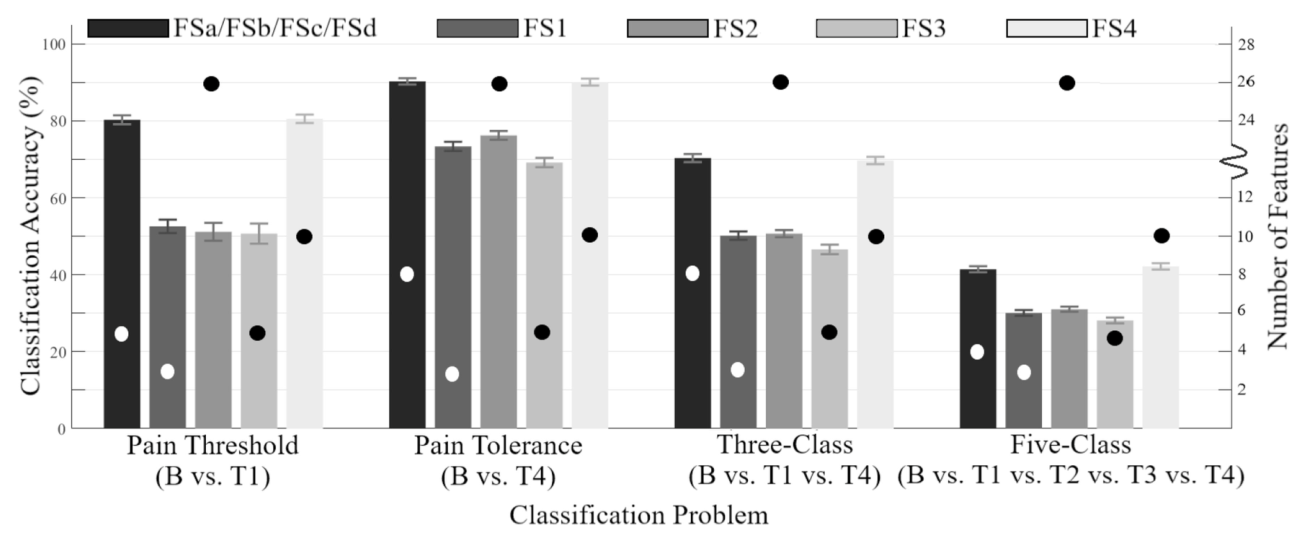
The compact SFS sets reached the following reported accuracies. Keeping the task beside the number is essential: separating baseline from the highest heat-pain level was much easier than resolving all five levels.
| Classification task | Features | Accuracy |
|---|---|---|
| Baseline vs. pain threshold (B / T1) | 5 | 80.3% |
| Baseline vs. pain tolerance (B / T4) | 8 | 90.3% |
| Three levels (B / T1 / T4) | 8 | 70.3% |
| All five levels (B / T1 / T2 / T3 / T4) | 4 | 41.4% |
Reported in Table 3 and Discussion, Section 4.1.1. These are results from the repeated trial-level splits described above; they are not leave-one-participant-out estimates.
The more revealing result was how redundant features affected selection. For baseline versus pain tolerance, UFS encountered an early local maximum at about 72.9%. Several highly ranked amplitude features added little beyond one another. Adding a lower-ranked corrugator correlation feature later raised accuracy to about 84.4%, because it supplied information the earlier features lacked.
That example explains why a ranking alone can mislead. A feature can be individually weaker yet become valuable in combination. It also explains why the stopping rule is part of the result: the early UFS maximum does not describe the best performance UFS could reach with more features.
Reading the figures
The feature chart gives the paper’s main argument a visual form. In this analysis, the objects being mapped are features, not participants. Each feature is represented by its values across the 8,500 trials.
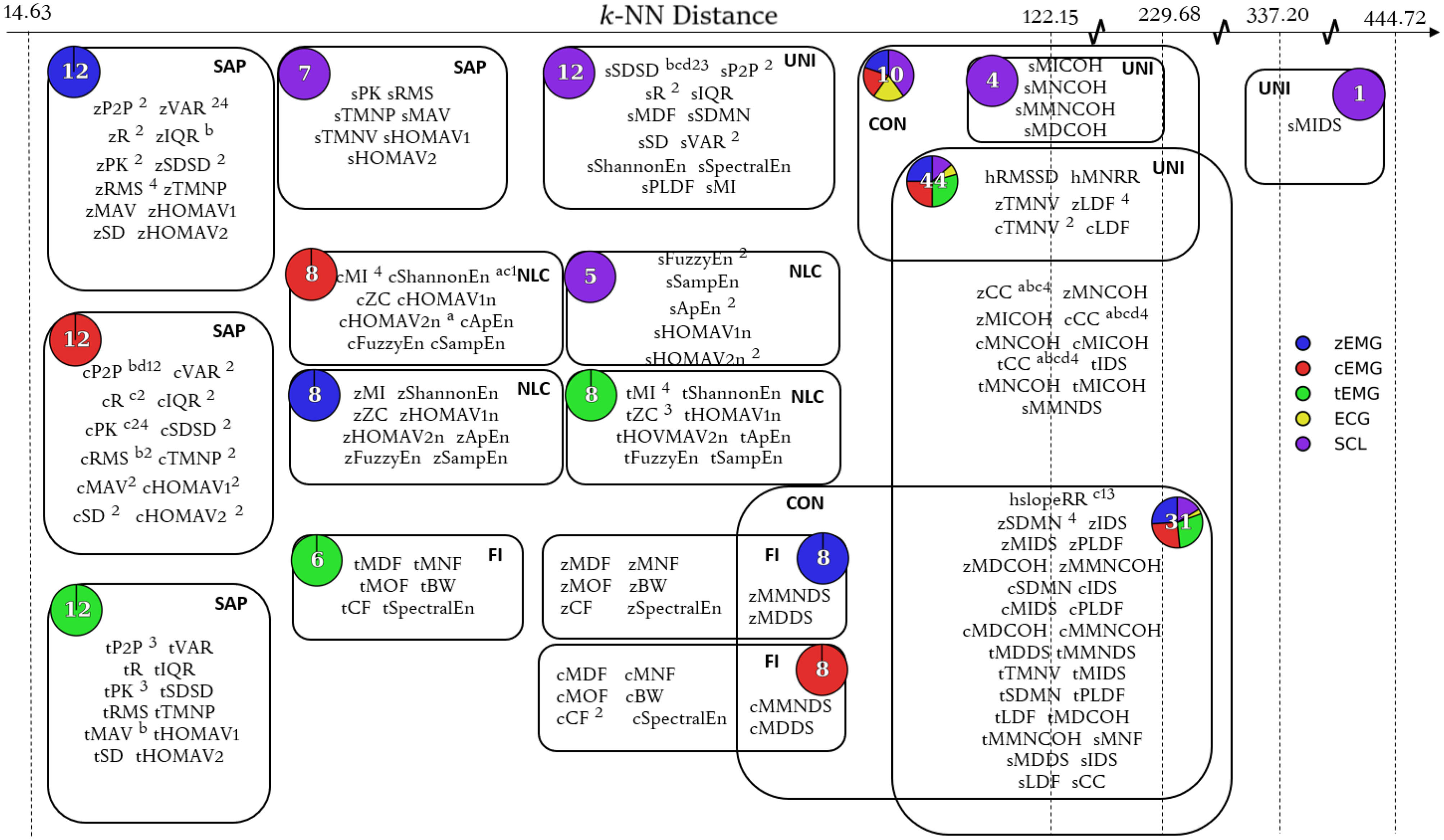
Read the chart in three steps. First, look for groups containing closely related amplitude measures. Next, look for features that occupy more distinct parts of the map. Finally, compare the sensor colors: some groups draw from one modality, while others contain a mixture. An edge indicates overlapping feature membership between Mapper clusters; it is not a causal connection between sensors.
The analysis organized features into five functional groups: signal amplitude and power, nonlinear complexity, frequency information, unique, and connecting. These describe how features behaved in the data, which need not match the categories implied by their formulas.
Why amplitude and variability features can overlap
For samples with mean μ, the squared root mean square equals the population variance plus the squared mean:
$$\mathrm{RMS}(x)^2 = \frac{1}{N}\sum_{i=1}^{N}x_i^2 = \mathrm{Var}(x) + \mu^2.$$
When an EMG window has a mean near zero, RMS and standard deviation become very similar. One is usually called an amplitude feature and the other a variability feature, but their labels can overstate the difference in what they measure. This identity uses the same 1/N convention for both quantities.
The ECG features did not form a group of their own. That suggested some of their information might be recoverable from EMG and SCL features. It is a useful sensor-design hypothesis, especially when fewer sensors would simplify a system, but it needs a direct removal-and-retest experiment before becoming a design rule.
The accuracy plot connects the feature-selection discussion to the four classification tasks. Bars use the left axis for accuracy; dots use the right axis for the number of selected features. Read the task groups separately: distinguishing baseline from the strongest stimulus is a different problem from assigning all five levels.
What the results do not establish
- New trials are not new people. Participants were represented across the training, validation, and test splits. The reported accuracies do not establish performance on a person excluded from model development.
- Heat-pain classification has a defined scope. These were controlled, brief stimuli with individually calibrated levels. Performance here does not establish continuous pain estimation or performance in a clinical setting. The paper itself notes that the accuracies may be inadequate for practical use.
- A feature’s context matters. Some consistently selected correlation features compare a recording with a pain-free baseline. Their usefulness must be considered alongside how that baseline would be obtained in the intended application.
- The map is an analysis, not a universal sensor ranking. Mapper depends on its distance metric, filter, and resolution. Only three ECG features were included. Their overlap in this study does not show that all cardiac information is redundant, or that ECG is unnecessary in every pain-recognition system.
Looking back
The lasting contribution is a way to reason about feature selection. Instead of asking only which list won, we can ask what information was represented, what was duplicated, and which choices persisted when the data changed. A changing feature name does not always mean an unstable underlying signal property.
For a follow-up study, three checks would make the next claims more informative: hold out entire participants, test whether the same relationships appear in an independent dataset, and remove a proposed redundant sensor before repeating selection and evaluation. Those are extensions suggested by this retrospective, rather than experiments reported in the 2019 paper.
Read further
Campbell, E., Phinyomark, A., and Scheme, E. (2019). Feature Extraction and Selection for Pain Recognition Using Peripheral Physiological Signals. Frontiers in Neuroscience, 13:437. doi:10.3389/fnins.2019.00437.
For the experimental protocol, read Sections 2.1–2.5 and Figure 1. For the reported numbers, see Tables 2–3 and Section 4.1.1. For the feature relationships, see Figures 3–4 and Sections 4.1.2–4.1.3. Read the complete paper.