Actor–critic methods: from a baseline to DDPG

REINFORCE uses a completed trajectory to judge an action. A critic provides a learned estimate that can be consulted during an episode. The actor decides what to do; the critic estimates the consequences. This post follows the course from a value baseline to bootstrapped actor–critic learning and then to continuous control with DDPG.

A baseline and a bootstrapped critic

With a state-value model \(V_\phi(s)\), REINFORCE can weight log probabilities by \(G_t-V_\phi(S_t)\). The value model can be trained against complete returns. This remains Monte Carlo learning for the value target; merely adding a second network does not introduce bootstrapping.

A one-step actor–critic instead uses $$y_t=R_{t+1}+\gamma(1-d_t)V_\phi(S_{t+1}),\qquad\delta_t=y_t-V_\phi(S_t).$$ The critic fits the detached target \(y_t\), and the actor uses the detached TD error as an advantage estimate. Terminology varies, but the course’s distinction is useful: does the learning target use a completed return or another estimate?

The TD error trades a noisy long-horizon return for an estimate that depends on the critic’s accuracy. It is not an exact advantage after every transition. A systematically wrong critic can systematically misdirect the actor.

When the TD error estimates an advantage

Let the critic be exact temporarily. The Bellman equation gives $$\mathbb E[R_{t+1}+\gamma V^\pi(S_{t+1})-V^\pi(S_t)\mid S_t=s,A_t=a]=Q^\pi(s,a)-V^\pi(s)=A^\pi(s,a).$$ Terminal continuation values are zero. Thus a one-step TD error can replace a complete return minus baseline in expectation when the value function is correct.

If the critic error is \(e(s)=V_\phi(s)-V^\pi(s)\), the conditional mean error in this advantage estimate is $$\gamma\mathbb E[e(S_{t+1})\mid s,a]-e(s).$$ The current-state term is action-independent and vanishes in the expected score-function update. The successor error can depend on the chosen action and bias the actor. This identifies precisely why a poor critic can be more consequential than a noisy but action-independent baseline.

For example, \(V_\phi(s)=3\), reward 1, successor value 4, and \(\gamma=0.9\) give \(\delta=1.6\). The actor receives positive feedback, but that signal would fall to −0.2 if the correct successor value were 2. A critic's generalization errors can therefore reverse the direction of policy learning, even with an accurate immediate reward.

Two losses, two responsibilities

For a sampled action, a local policy-loss contribution is \(-\log\pi_\theta(a\mid s)\,\operatorname{stopgrad}(\delta)\). The critic loss is \((V_\phi(s)-\operatorname{stopgrad}(y))^2\). The state-sampling and time weighting must match the chosen policy objective, as in the preceding REINFORCE derivation.

Detaching the advantage prevents the policy loss from changing the critic merely to make its own weight convenient. Detaching the target prevents the value update from chasing gradients through the next-state estimate. Shared actor–critic encoders require an explicit combined-loss design; separate networks make the roles easier to inspect.

For a categorical policy, entropy is \(H(\pi)=-\sum_a\pi(a\mid s)\log\pi(a\mid s)\). Subtracting \(\beta H\) from a minimized policy loss encourages a less concentrated distribution. It encourages exploration; it does not certify uncertainty or guarantee that all useful actions will be visited.

Several-step advantages bridge Monte Carlo and one-step critics

The n-step return from the TD post supplies an advantage estimate \(\hat A_t^{(n)}=G_t^{(n)}-V_\phi(S_t)\). With values held fixed during the calculation, it equals a discounted sum of TD errors. This allows a choice between using mostly observed rewards and relying heavily on a short bootstrap.

A commonly used extension is generalized advantage estimation. For a segment ending at \(T\), its backward recursion is $$\hat A_t^{\mathrm{GAE}}=\delta_t+\gamma\lambda\hat A_{t+1}^{\mathrm{GAE}},\qquad\hat A_T^{\mathrm{GAE}}=0.$$ At true episode boundaries use zero continuation; at a collection cutoff the final TD error can bootstrap, but the recursion must not flow into a reset episode. With \(\lambda=0\) we recover one-step TD. With \(\lambda=1\) and a completed episode, the sum telescopes to \(G_t-V_\phi(S_t)\). Intermediate values trade longer sampled credit assignment against reliance on the learned critic. This is an extension of the course's bridge, not a claim that the displayed DDPG kernel implements GAE.

Generalized advantage estimation: Schulman and colleagues

Why continuous actions change the critic interface

A DQN output vector is convenient when we can enumerate actions. It is awkward when the action is a motor torque that can take any value in an interval. Discretizing multiple actuators makes the action grid grow rapidly, just as observation grids did earlier in the series.

Deep Deterministic Policy Gradient, or DDPG, uses an actor \(a=\mu_\theta(s)\) and a critic \(Q_\phi(s,a)\). The critic takes the action as an input and returns one scalar. The actor proposes an action without exhaustively maximizing the critic over a continuous action space.

For bounded actions, a tanh output \(u\) can be mapped to the environment by $$a=\frac{a_{\max}+a_{\min}}2+\frac{a_{\max}-a_{\min}}2\odot u.$$ Apply these bounds per action dimension. A fixed −1 to 1 convention is useful internally, but is not automatically the physical action range.

DDPG: Lillicrap and colleagues

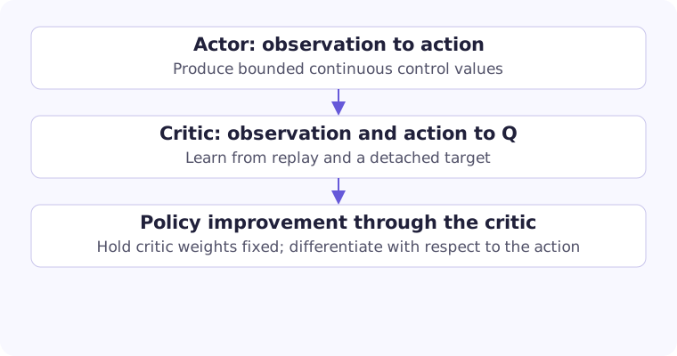
These two original diagrams show the change in interfaces: the actor maps a state to a bounded action, while the critic takes both a state and an action to produce a scalar Q estimate. The action is therefore an input to the critic, rather than an index into a vector of outputs.

A continuous policy can also be stochastic

Before specializing to DDPG, consider a scalar Gaussian policy with learned mean and standard deviation: $$\log\pi_\theta(a\mid s)=-\frac{(a-\mu_\theta(s))^2}{2\sigma_\theta(s)^2}-\log\sigma_\theta(s)-\frac12\log(2\pi).$$ Its mean score is \(\partial\log\pi/\partial\mu=(a-\mu)/\sigma^2\). Positive advantage pushes the mean toward a sampled action, scaled by the distribution's variance. This is still the stochastic policy-gradient mechanism, now with a density instead of discrete probabilities.

Continuous actions therefore do not force us to use deterministic policies. DDPG makes that design choice to optimize a proposed action through a differentiable critic. SAC will return to learned distributions, with bounded samples and an explicit entropy objective. Keeping these alternatives separate prevents confusing continuous action spaces with one particular algorithm family.

The DDPG critic target and actor gradient

DDPG uses replay and target copies of both networks. For a replayed transition, $$y=r+\gamma(1-d)Q_{\bar\phi}(s^{\prime},\mu_{\bar\theta}(s^{\prime})).$$ Fit \(Q_\phi(s,a)\) to this detached target. The current prediction uses the recorded action; the target uses an action proposed at the next state by the target actor.

The actor minimizes $$L_\mu=-\mathbb E_{s\sim\mathcal D}[Q_\phi(s,\mu_\theta(s))].$$ Its gradient flows through the critic’s action input and back into the actor: $$\nabla_\theta Q_\phi(s,\mu_\theta(s))=\nabla_aQ_\phi(s,a)\vert_{a=\mu_\theta(s)}\,\nabla_\theta\mu_\theta(s).$$ The environment need not be differentiable because this derivative passes through the learned critic.

During this actor update, hold critic parameters fixed while retaining differentiation with respect to its action input. Wrapping the entire critic call in no_grad would remove the very path the actor needs. The actor is improving the critic’s estimate of return, so inaccurate value gradients remain a central limitation.

What distribution belongs in a deterministic policy gradient?

For the discounted start-state objective, define the unnormalized occupancy \(\rho^\mu(s)=\sum_{t\ge0}\gamma^t\Pr(S_t=s\mid\mu)\). Under suitable differentiability and regularity assumptions, the deterministic policy-gradient theorem gives $$\nabla_\theta J=\int\rho^\mu(s)\,\nabla_\theta\mu_\theta(s)\,\nabla_a Q^\mu(s,a)\big|_{a=\mu_\theta(s)}\,ds.$$ The theorem accounts for future state visitation through the value function and occupancy; naively differentiating only the immediate reward would miss that effect.

Practical DDPG substitutes a learned critic and replay-buffer states. Its actor loss is consequently a surrogate averaged over the replay distribution, not automatically an unbiased estimate of that exact on-policy start-state gradient. Adequate coverage and useful critic action derivatives are essential assumptions behind the approximation. Off-policy replay permits learning from exploratory behavior, but does not remove this distribution mismatch.

For a simple local example, suppose \(Q(s,a)=5-(a-0.6)^2\) and the actor currently proposes 0.2. The action derivative is \(-2(a-0.6)=0.8\), so a small ascent step increases the proposed action toward 0.6. If the actor uses \(a=m+c\tanh z_\theta(s)\), then $$\nabla_\theta a=c(1-\tanh^2z_\theta(s))\nabla_\theta z_\theta(s).$$ Near saturation the gradient can be small even when the critic requests a substantial change. This makes action scaling and the actor's parameterization part of the optimization problem.

Deterministic policy-gradient theorem: Silver and colleagues

The two update steps

This kernel assumes separate actor and critic networks, target copies initialized from them, and matching optimizers. Actors return actions already scaled to environment bounds; critics return [B, 1]. All batch tensors must share a device. Collection, replay sampling, exploration noise, and target updates surround this kernel.

import torch
from torch.nn import functional as F

def ddpg_step(actor, critic, target_actor, target_critic,
              actor_optimizer, critic_optimizer,
              states, actions, rewards, next_states, terminated,
              gamma=0.99):
    with torch.no_grad():
        next_q = target_critic(next_states, target_actor(next_states))
        y = rewards + gamma * (~terminated.bool()).float() * next_q.squeeze(-1)
    critic_loss = F.mse_loss(critic(states, actions).squeeze(-1), y)
    critic_optimizer.zero_grad()
    critic_loss.backward()
    critic_optimizer.step()

    flags = [p.requires_grad for p in critic.parameters()]
    for p in critic.parameters():
        p.requires_grad_(False)
    try:
        actor_loss = -critic(states, actor(states)).mean()
        actor_optimizer.zero_grad()
        actor_loss.backward()
        actor_optimizer.step()
    finally:
        for p, flag in zip(critic.parameters(), flags):
            p.requires_grad_(flag)
    return critic_loss.item(), actor_loss.item()

A target update is a separate operation. With a small mixing coefficient τ, replace each target parameter by (1 − τ) times its current value plus τ times the corresponding online parameter. Apply that rule to both the actor and critic target copies. Target parameters do not receive optimizer steps.

Two learning rates and two slowly moving copies

With separate networks, a critic step minimizes \(\frac1B\sum_i(Q_\phi(s_i,a_i)-y_i)^2\), while an actor step minimizes \(-\frac1B\sum_iQ_\phi(s_i,\mu_\theta(s_i))\). These objectives have different units and gradient paths; they need not use the same learning rate. If the actor moves quickly relative to the critic's ability to evaluate it, it can repeatedly chase value errors.

The target copies obey $$\bar\phi\leftarrow(1-\tau)\bar\phi+\tau\phi,\qquad\bar\theta\leftarrow(1-\tau)\bar\theta+\tau\theta.$$ The behaviour action can be written \(a_{\mathrm{env}}=\operatorname{clip}(\mu_\theta(s)+\epsilon,a_{\min},a_{\max})\), with a specified exploration process \(\epsilon\). The critic's current-state input is this executed action, not an unperturbed action that the environment never received. The target actor supplies the hypothetical next action used to evaluate future deterministic behavior.

Exploration and an honest experiment

A deterministic actor gives the same action for the same state. During training, add exploration noise and clip to the action bounds before passing the action to the environment. Store the action actually executed. The course’s continuous LunarLander example illustrates this setup; the learned actor can be evaluated without that added noise.

Compare training return with separate evaluation return and inspect whether actions spend excessive time at their bounds. Large critic predictions combined with poor behaviour may indicate that the actor is exploiting estimation errors. Increasing policy-update frequency can make that problem worse rather than solve it.

A continuous policy is a representation choice, not a guarantee of smooth, safe, or optimal behaviour. DDPG provides the machinery to optimize continuous outputs through a critic. The next post examines how TD3 limits specific critic errors and how SAC changes the objective to include policy entropy.

Next: TD3 and soft actor–critic

Adapted from my reinforcement learning course: module 08, slides 6–16 and DDPG_lunarlander.py. The worked examples in this post are teaching examples, not benchmark results.