But do we really need to wait for an entire episode?
Monte Carlo learning implicitly assumes that to get a good estimate of the long-term return, we need to look all the way to the end of the episode. But we also spent a lot of time establishing something important:If the problem satisfies the Markov property, the next state and reward depend only on the current state and action.If that is true (or true enough), then perhaps we can get away with not waiting until the end of the episode. Maybe we can learn during the episode — one transition at a time — instead of only after it. That idea leads to Temporal Difference (TD) learning.
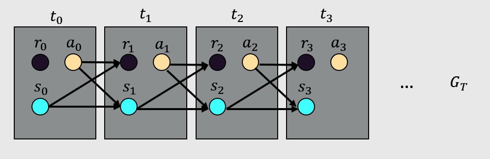
From Monte Carlo Updates to Temporal Difference Updates
Monte Carlo policy evaluation updated the value of a state using: $$ V(s_t) \leftarrow V(s_t) + \alpha \big[ G_t - V(s_t) \big], $$ where \(G_t\) is computed using full-episode returns. But if we want to learn every time step, we need a way to replace \(G_t\) with something available immediately. Note that: $$ G_t = R_{t+1} + \gamma G_{t+1}, $$ and the first part — the immediate reward — is always known after a single transition. For the rest of the return, we don’t have the true value… but we do have our current estimate of the next state’s value. Temporal Difference learning simply uses that: $$ G_t \approx R_{t+1} + \gamma V(s_{t+1}). $$ Plugging this approximation into the Monte Carlo update gives: $$ V(s_t) \leftarrow V(s_t) + \alpha \big[ R_{t+1} + \gamma V(s_{t+1}) - V(s_t) \big]. $$ The term: $$ \delta_t = R_{t+1} + \gamma V(s_{t+1}) - V(s_t) $$ is called the Temporal Difference error. It measures how “surprised” we are by what actually happened relative to what we previously believed. This learning procedure is called TD(0) because it uses only a single step of lookahead. It learns online, incrementally, and does not require a model.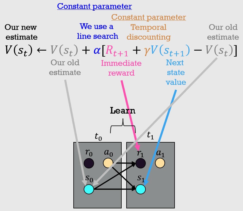
A sampled Bellman backup and its source of bias
Fix the current value table while taking an expectation over the next transition. Under policy \(\pi\), $$\mathbb E[\delta_t\mid S_t=s]=(T^\pi V)(s)-V(s).$$ A TD error is therefore a noisy estimate of the current Bellman residual. It need not have mean zero until the table reaches the fixed point. Monte Carlo instead samples a complete return whose expectation is \(V^\pi(s)\), independent of the current table.
For a nonterminal transition, suppose \(V(s)=2\), \(V(s')=4\), \(r=1\), and \(\gamma=0.9\). The TD target is 4.6 and the error is 2.6; with learning rate 0.1, the new prediction is 2.26. If the observed remainder of the episode later totals a discounted return of 7, MC would have updated toward 7. TD can learn sooner, but its target depends on the accuracy of the successor estimate. The familiar bias–variance trade-off concerns that target, not a promise that TD is better on every task.
From State-Values to Action-Values
So far we discussed updating the state value function \(V(s)\). But acting optimally requires reasoning about actions, so TD learning is commonly applied to the action-value function: $$ Q(s,a). $$ Once we work with \(Q(s,a)\), we can fold the policy directly into the update rule. This is where SARSA appears as a natural TD control algorithm.Several steps connect TD back to Monte Carlo
We need not choose only between one transition and a whole episode. If \(n\) steps are available before termination, an n-step return is $$G_t^{(n)}=\sum_{k=0}^{n-1}\gamma^kR_{t+k+1}+\gamma^nV(S_{t+n}).$$ If the episode terminates sooner, stop the reward sum there and omit the bootstrap. Setting \(n=1\) recovers TD(0); extending to the episode's end recovers the Monte Carlo return. Longer targets depend on more observed rewards and on a more distant, more heavily discounted estimate.
For a fixed table and a segment containing \(n\) nonterminal steps, the errors telescope: $$G_t^{(n)}-V(S_t)=\sum_{k=0}^{n-1}\gamma^k\delta_{t+k}.$$ Each intermediate value appears once positively and once negatively. This identity explains how later prediction errors can assign credit to earlier states. Online table changes complicate the exact equality, so it is best understood first with values held fixed over the calculation.
SARSA: On-Policy Temporal Difference Learning
SARSA is named after the sequence it uses in its update: (State, Action, Reward, Next State, Next Action) At each time step:- We are in state \(s_t\).
- We pick action \(a_t\) using our current (usually ε-greedy) policy.
- We observe reward \(R_{t+1}\) and next state \(s_{t+1}\).
- We pick the next action \(a_{t+1}\) from the same policy.
- We update \(Q(s_t,a_t)\) toward the one-step TD target that uses \(Q(s_{t+1}, a_{t+1})\).
Averaging over the next action gives Expected SARSA
SARSA samples the next action from its policy and uses that action's Q-value. Expected SARSA averages over the same policy instead: $$y_{\mathrm{ES}}=r+\gamma(1-d)\sum_a\pi(a\mid s')Q(s',a).$$ Here \(d=1\) means true termination. This removes the randomness of sampling the next action conditional on \(s'\), while randomness in the reward and successor state remains.
For next-state values 5 and 1 with epsilon-greedy \(\varepsilon=0.2\), the two probabilities are 0.9 and 0.1. With \(r=0\) and \(\gamma=0.9\), SARSA's sampled target is 4.5 or 0.9; Expected SARSA's target is 4.14. Q-learning instead uses 4.5 regardless of which action exploration actually chooses. This difference explains why SARSA can value a route according to the risks of its continuing exploration, while Q-learning evaluates a greedy continuation.
Q-learning: learning a greedy target policy
Q-learning has a similar structure to SARSA, but makes a key change: instead of updating toward the value of the actual next action \(a_{t+1}\), it updates toward the value of the best possible next action: $$ Q(s_t,a_t) \leftarrow Q(s_t,a_t) + \alpha \Big[ R_{t+1} + \gamma \max_{a'} Q(s_{t+1}, a') - Q(s_t,a_t) \Big]. $$ This makes Q-learning an off-policy TD control algorithm:- The behavior policy can be ε-greedy (or anything that explores enough).
- The target in the update always assumes a greedy policy in the future (via the max over actions).
What the tabular convergence claim requires
In a finite discounted MDP with bounded rewards, tabular Q-learning converges under suitable sampling and step-size conditions: every state-action pair must be visited infinitely often, and its own step sizes satisfy $$\sum_n\alpha_n(s,a)=\infty,\qquad\sum_n\alpha_n(s,a)^2<\infty.$$ The first condition permits correction of initial errors; the second damps accumulated noise. A constant learning rate, a finite run, and a coarse observation digitizer do not meet this theorem merely because the code contains a max operator.
Q-learning is off-policy because its target uses a greedy action even when its behaviour explores. This is separate from optimism through deliberately high initial values or confidence bonuses. A noisy maximum can also overestimate values; that statistical effect motivates Double DQN later in the series. None of these uses of optimism implies that a Q-learning controller always takes a safe or high-reward action during training.
Q-learning tutorial: CartPole control in Python
We will work with a tabular Q-learning agent. That means we need:- categorical (discrete) states,
- a table \(Q(s,a)\) for each discrete state–action pair,
- an exploration strategy (ε-greedy), and
- a training loop over many episodes.
Episode boundaries belong in the target
The terminal target is just the reward: $$y=r+\gamma(1-d)\max_aQ(s',a).$$ Bootstrapping after genuine failure adds a continuation that the task does not have. Conversely, an external collection time limit may stop a rollout while the underlying task could continue. The loop then resets, but the target can still bootstrap from the final observation. Keep the rollout-ending flag distinct from the true-termination flag used in the equation.
State aggregation introduces another limitation. The digitizer maps an observation to a bin \(\bar s=\phi(s)\), so different velocities or angles can share one Q entry. If their next-bin distributions differ, the aggregate process need not be exactly Markov. The ten edge values in each dimension below produce eleven possible indices, including the two outer intervals, for \(11^4\times2=29,282\) Q entries. This representation saves computation by treating observations as equivalent; it does not prove that the equivalence preserves the optimal policy.
Gymnasium: termination, truncation, and bootstrap targets
1. Imports and entry point: how the simulation runs
Imports and __main__ block
import gymnasium as gym
import matplotlib.pyplot as plt
import numpy as np

def plot_learning_curve(scores, x):
    running_avg = np.zeros(len(scores))
    for i in range(len(running_avg)):
        running_avg[i] = np.mean(scores[max(0, i-100):(i+1)])
    plt.plot(x, running_avg)
    plt.title('Running average of previous 100 scores')
    plt.savefig('qlearning_control_cartpole.png')


if __name__ == '__main__':
    env = gym.make('CartPole-v1')
    n_games = 50000
    eps_dec = 2 / n_games

    digitizer = CartPoleStateDigitizer()
    agent = Agent(
        alpha=0.01,
        gamma=0.99,
        n_actions=2,
        epsilon=1.0,
        eps_min=0.01,
        eps_dec=eps_dec,
        state_space=digitizer.states
    )

    scores = []

    for i in range(n_games):
        observation, _ = env.reset()
        done = False
        score = 0
        state = digitizer.digitize(observation)

        while not done:
            action = agent.choose_action(state)
            observation_, reward, terminated, truncated, info = env.step(action)
            done = terminated or truncated
            state_ = digitizer.digitize(observation_)
            agent.learn(state, action, reward, state_, terminated)
            state = state_
            score += reward

        if i % 5000 == 0:
            print('episode', i, 'score %.1f' % score, 'epsilon %.2f' % agent.epsilon)

        agent.epsilon_decrement()
        scores.append(score)

    x = [i + 1 for i in range(n_games)]
plot_learning_curve(scores, x)- Create the
CartPole-v1environment. - Set the number of training episodes (
n_games = 50000). - Set the rate at which we decay ε (
eps_dec), going from 1.0 down to around 0.01 over training. - Instantiate the
CartPoleStateDigitizer(to discretize continuous observations). - Instantiate the
Agentwith learning ratealpha, discountgamma, etc. - For each episode:
- Reset the env, digitize the initial observation into a discrete state.
- Loop until episode termination:
- Choose an action via ε-greedy policy.
- Step the environment, get next observation and reward.
- Digitize the new observation into next state.
- Call
agent.learn(state, action, reward, state_, terminated)to apply the Q-learning update. - Move to the next state and accumulate episode reward.
- Periodically print episode stats and current ε.
- Decay ε via
agent.epsilon_decrement(). - Store each episode’s total score.
- After training, plot the running average score over the last 100 episodes.
2. Digitizing CartPole state: making tabular Q-learning possible
CartPole observations are continuous: \((x, \dot x, \theta, \dot\theta)\). A tabular Q-learner needs discrete state indices. TheCartPoleStateDigitizer class discretizes each dimension into bins and returns a tuple of bin indices. CartPoleStateDigitizer
class CartPoleStateDigitizer():
    def __init__(self, bounds=(2.4, 4, 0.209, 4), n_bins=10):
        self.position_space = np.linspace(-1 * bounds[0], bounds[0], n_bins)
        self.velocity_space = np.linspace(-1 * bounds[1], bounds[1], n_bins)
        self.pole_angle_space = np.linspace(-1 * bounds[2], bounds[2], n_bins)
        self.pole_velocity_space = np.linspace(-1 * bounds[3], bounds[3], n_bins)
        self.states = self.get_state_space()

    def get_state_space(self):
        states = []
        for i in range(len(self.position_space) + 1):
            for j in range(len(self.velocity_space) + 1):
                for k in range(len(self.pole_angle_space) + 1):
                    for l in range(len(self.pole_velocity_space) + 1):
                        states.append((i, j, k, l))
        return states

    def digitize(self, observation):
        x, x_dot, theta, theta_dot = observation
        cart_x = int(np.digitize(x, self.position_space))
        cart_xdot = int(np.digitize(x_dot, self.velocity_space))
        pole_theta = int(np.digitize(theta, self.pole_angle_space))
        pole_thetadot = int(np.digitize(theta_dot, self.pole_velocity_space))
return (cart_x, cart_xdot, pole_theta, pole_thetadot)- Bin edges: each physical quantity is sliced into
n_binsequally spaced edges; digitize also includes intervals outside those bounds. - State space:
self.statesenumerates all tuples \((i,j,k,l)\) of bin indices; this is the discrete state space used to initialize the Q-table. - digitize:
np.digitizemaps each real-valued observation component to an integer bin index. The result is a categorical state suitable for tabular Q-learning.
3. The Agent: Q-table, ε-greedy policy, and the Q-learning update
TheAgent encapsulates the Q-learning logic: it holds the Q-table, chooses actions ε-greedily, and applies the update: $$ Q(s_t,a_t) \leftarrow Q(s_t,a_t) + \alpha \Big[ R_{t+1} + \gamma \max_{a'} Q(s_{t+1}, a') - Q(s_t,a_t) \Big]. $$ Agent class
class Agent():
    def __init__(self, alpha, gamma, n_actions, state_space,
                 epsilon=1, eps_dec=5e-4, eps_min=0.01):
        self.alpha = alpha
        self.gamma = gamma
        self.state_space = state_space
        self.actions = [i for i in range(n_actions)]
        self.epsilon = epsilon
        self.eps_dec = eps_dec
        self.eps_min = eps_min
        self.Q = {}
        self.init_Q()

    def init_Q(self):
        for state in self.state_space:
            for action in self.actions:
                self.Q[(state, action)] = 0.0

    def max_action(self, state):
        actions = np.array([self.Q[(state, a)] for a in self.actions])
        action = np.argmax(actions)
        return action

    def choose_action(self, state):
        if np.random.random() < self.epsilon:
            return np.random.choice(self.actions)
        return self.max_action(state)

    def epsilon_decrement(self):
        if self.epsilon > self.eps_min:
            self.epsilon = max(self.eps_min, self.epsilon - self.eps_dec)
        else:
            self.epsilon = self.eps_min

    def learn(self, state, action, reward, state_, terminated):
        a_max = self.max_action(state_)
        q_next = reward + self.gamma * (not terminated) * self.Q[(state_, a_max)]
self.Q[(state, action)] += self.alpha * (q_next - self.Q[(state, action)])- Q-table:
self.Q[(state, action)]represents \(Q(s,a)\). - Action space:
self.actionsis the set of possible actions \(\mathcal{A}\). - Greedy action:
max_action(state)computes \(\arg\max_a Q(s,a)\). - ε-greedy policy:
choose_action:- With probability ε, pick a random action (exploration).
- Otherwise, pick the greedy action (exploitation).
- Annealing ε:
epsilon_decrementslowly reduces ε from 1.0 down toeps_min, shifting from exploration to exploitation. - Learning step:
learn:a_max = self.max_action(state_)computes \(\arg\max_{a'} Q(s_{t+1}, a')\).q_next = reward + self.gamma * (not terminated) * self.Q[(state_, a_max)]computes the target \(R_{t+1}+\gamma(1-d_t)\max_{a'}Q(s_{t+1},a')\), with zero continuation after termination.self.Q[(state, action)] += self.alpha * (q_next - self.Q[(state, action)])applies the Q-learning update.
learn: we would pass the actual next action \(a_{t+1}\) into learn and update toward \(R_{t+1} + \gamma Q(s_{t+1}, a_{t+1})\) instead of using \(\max_{a'} Q(s_{t+1}, a')\). The existing figure below records the earlier course run. The corrected example above uses CartPole-v1 and explicit terminal masking; this historical curve is not a rerun of that updated code: 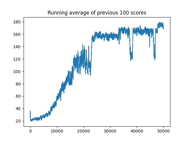
Summary
- Monte Carlo methods learn only after full episodes; TD methods learn every time step.
- SARSA is an on-policy TD control algorithm: $$Q(s_t,a_t) \leftarrow Q(s_t,a_t) + \alpha [R_{t+1} + \gamma Q(s_{t+1},a_{t+1}) - Q(s_t,a_t)].$$
- Q-learning is an off-policy TD control algorithm: $$Q(s_t,a_t) \leftarrow Q(s_t,a_t) + \alpha [R_{t+1} + \gamma \max_{a'}Q(s_{t+1},a') - Q(s_t,a_t)].$$
- Tabular Q-learning requires discrete states; we used a digitizer to approximate CartPole’s continuous dynamics with a finite MDP.
- The Q-learning update is implemented in
Agent.learn, directly matching the mathematical form.