DQN learns action values and uses them to choose actions. REINFORCE changes the object we train: the network represents the policy itself. We still need experience to discover which choices work, but now the update changes the probability of those choices directly.
An output vector with a different meaning
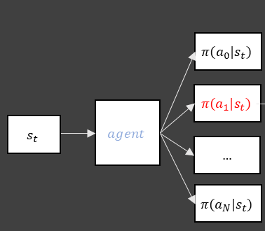
For a discrete action set, a policy network produces logits \(z_\theta(s)\). Their softmax defines \(\pi_\theta(a\mid s)\), the probability of sampling each action. These outputs are not Q-values. A probability of 0.8 means that the policy selects an action frequently; it does not mean that the action has an expected return of 0.8.
The course’s LunarLander example uses eight observations, two hidden layers of 128 units, and four action outputs. During training it samples an action from a categorical distribution. Selecting the largest logit every time would replace that sampling policy with a different behaviour policy.
Sampling provides exploration, but does not guarantee adequate coverage. A policy can become concentrated on a poor action before it has gathered enough useful evidence. Stochastic action selection also does not, by itself, solve partial observability; missing information may require history or a recurrent state representation.
The policy-network portion of the original slide highlights the probability of the action that was sampled. Keeping that particular output connected to its computation graph is what allows the later return-weighted update to change the policy.
Turning logits into a differentiable policy
For \(K\) actions, softmax defines $$\pi_\theta(a\mid s)=\frac{\exp z_{\theta,a}(s)}{\sum_{j=1}^K\exp z_{\theta,j}(s)},\qquad\log\pi_\theta(a\mid s)=z_{\theta,a}(s)-\log\sum_j\exp z_{\theta,j}(s).$$ Adding the same constant to every logit changes no probability. Stable implementations exploit this by subtracting the largest logit before exponentiating. The log-sum-exp form is also why directly computing log probabilities is preferable to taking the logarithm of a probability already rounded toward zero.
We do not differentiate the discrete action sample itself. The sample tells us which log probability to differentiate. This score-function approach works even when the environment and categorical choice are not differentiable. Its price is sampling variance: we need evidence about how sampled choices relate to later return.
Keep the trajectory, then work backwards
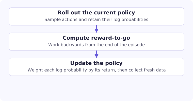
After a complete episode, compute the reward-to-go for each decision: $$G_t=R_{t+1}+\gamma G_{t+1},\qquad G_T=0.$$ This includes all subsequent discounted rewards, not just the final reward. The course script computes every suffix separately; one reverse pass gives the same values in linear time.
def reward_to_go(rewards, gamma=0.99):
    returns = [0.0] * len(rewards)
    running = 0.0
    for t in range(len(rewards) - 1, -1, -1):
        running = rewards[t] + gamma * running
        returns[t] = running
    return returns

print(reward_to_go([1.0, 0.0, 2.0], gamma=0.9))
# [2.62, 1.8, 2.0]
The first decision receives credit for the entire remaining sequence. The final decision receives only the reward that follows it. That credit is noisy: later actions and environment randomness also contributed to the result. REINFORCE relies on averaging sampled evidence, not on identifying a uniquely causal action from one successful episode.
Define the objective before assigning credit
Let \(\rho_0\) be the fixed distribution of starting states. For an episode with \(T\) decisions, define \(F(\tau)=\sum_{t=0}^{T-1}\gamma^tR_{t+1}\) and \(J(\theta)=\mathbb E_{\tau\sim p_\theta}[F(\tau)]\). This averages over initial states, sampled actions, and environment outcomes. A finite horizon can be included in the state; a random terminal time can be represented by padding subsequent rewards with zeros.
The policy is held fixed while each trajectory is collected. Changing its parameters halfway through a rollout changes the trajectory distribution and requires corresponding bookkeeping in a likelihood-based derivation. Similarly, averaging each episode's total gradient over a batch of episodes is different from dividing every episode by its own length: the latter gives short and long trajectories different relative weights.
Why the log probability appears
Let a trajectory be \(\tau\), with probability \(p_\theta(\tau)\). The identity \(\nabla_\theta p_\theta=p_\theta\nabla_\theta\log p_\theta\) lets us differentiate an expectation using sampled trajectories. When the environment dynamics do not depend on the policy parameters, the parameter-dependent terms in its log probability are the chosen actions’ log probabilities.
For the discounted start-state objective \(J(\theta)=\mathbb E[\sum_t\gamma^tR_{t+1}]\), a sampled gradient estimator is $$\hat g=\sum_t\gamma^tG_t\nabla_\theta\log\pi_\theta(A_t\mid S_t).$$ Rewards before a decision can be removed from its weight because that decision cannot affect them. With \(\gamma=1\), this becomes the familiar undiscounted episodic estimator.
An optimizer that minimizes a loss can implement ascent on that estimator using $$L=-\sum_t\gamma^tG_t\log\pi_\theta(A_t\mid S_t).$$ The minus sign matters. Minimizing the positive log-probability product would reverse the intended update. The additional \(\gamma^t\) matches the stated discounted start-state objective; practical implementations sometimes omit it, including the course example.
The update size cannot be read from the loss value alone. For a softmax logit \(z_j\), \(\partial\log\pi(a\mid s)/\partial z_j=\mathbf 1[j=a]-\pi(j\mid s)\). A favourable sampled action is pushed up relative to its alternatives, with the change governed by this derivative and the return weight.
Deriving the trajectory gradient step by step
With a joint reward-transition model, a trajectory has probability $$p_\theta(\tau)=\rho_0(s_0)\prod_{t=0}^{T-1}\pi_\theta(a_t\mid s_t)\,p(s_{t+1},r_{t+1}\mid s_t,a_t).$$ Only the policy factors depend on \(\theta\). Under the usual conditions allowing differentiation inside the expectation, $$\begin{aligned}\nabla_\theta J&=\int F(\tau)\nabla_\theta p_\theta(\tau)\,d\tau\\&=\mathbb E\left[F(\tau)\sum_t\nabla_\theta\log\pi_\theta(A_t\mid S_t)\right].\end{aligned}$$ For discrete trajectories the integral is a sum. No derivative of the environment model appears; its influence is already represented by which trajectories occur.
Now fix the history immediately before action \(A_t\). Any earlier reward is constant conditional on that history, while the conditional mean score is zero: $$\mathbb E[\nabla_\theta\log\pi_\theta(A_t\mid S_t)\mid\text{history}]=\sum_a\nabla_\theta\pi_\theta(a\mid S_t)=0.$$ Earlier rewards therefore contribute zero in expectation and can be removed from the weight. The remaining discounted suffix is \(\sum_{k=t}^{T-1}\gamma^kR_{k+1}=\gamma^tG_t\), yielding the estimator above. Removing irrelevant past rewards preserves the expected gradient while avoiding one source of noise.
As a local numerical example, take two action probabilities \((0.25,0.75)\), sample action 0, and suppose its advantage weight is 2 at time zero. The ascent direction for the two logits is \(2(1-0.25,-0.75)=(1.5,-1.5)\). A small ascent step raises the sampled action's probability relative to the other. With advantage −2, the direction reverses. Shared network parameters can also change probabilities at other states, so this local calculation does not predict the complete post-update policy.
A compact episode update
The following PyTorch functions show the parts that differ from DQN. The policy must return one vector of logits for the observation. Collect log_probs and rewards for one complete episode without changing policy parameters during collection; then call finish_episode. The reward_to_go helper above is also required.
import torch
from torch.distributions import Categorical

def sample_action(policy, observation):
    parameter = next(policy.parameters())
    state = torch.as_tensor(observation, dtype=parameter.dtype,
                            device=parameter.device)
    distribution = Categorical(logits=policy(state))
    action = distribution.sample()
    return action.item(), distribution.log_prob(action)

def finish_episode(optimizer, log_probs, rewards, gamma=0.99):
    logp = torch.stack(log_probs)
    returns = torch.tensor(reward_to_go(rewards, gamma),
                           dtype=logp.dtype, device=logp.device)
    time_weights = gamma ** torch.arange(len(rewards),
                                         device=logp.device)
    loss = -(time_weights * returns * logp).sum()
    optimizer.zero_grad()
    loss.backward()
    optimizer.step()
    return loss.item()
Categorical(logits=...) handles normalization and log probabilities together. Keep the log-probability tensors attached to their computation graphs until the update; converting them to Python numbers would destroy the gradient path. Clear the episode’s lists afterward, and collect fresh data with the updated policy.
This is an on-policy episode update, not a replay-buffer update. Repeatedly optimizing old trajectories changes the relationship between the sampling policy and the policy being differentiated. Importance sampling or other carefully specified corrections would be needed for a different data-reuse scheme.
Better than what? Introduce a baseline
If every return is positive, a simple sampled update reinforces even a relatively disappointing choice. A state-dependent baseline gives the weight a useful reference: $$\hat A_t=G_t-b(S_t).$$ For example, returns of 10 and 12 relative to a baseline of 11 give weights of −1 and +1.
An action-independent baseline leaves the expected score-function gradient unchanged: $$\mathbb E_{a\sim\pi}[b(s)\nabla_\theta\log\pi(a\mid s)]=b(s)\nabla_\theta\sum_a\pi(a\mid s)=0.$$ A suitable baseline can reduce variance. A learned state-value predictor is a natural choice, provided the policy loss treats the baseline as a fixed weight during that update.
That does not mean any normalization is equivalent to a baseline. Subtracting a sample-dependent mean or dividing by the episode’s standard deviation changes the finite-sample estimator. Those can be useful practical choices, but they should be described rather than silently added to a derivation.
A value baseline is useful, but not uniquely variance-optimal
The true advantage is \(A^\pi(s,a)=Q^\pi(s,a)-V^\pi(s)\), with $$\sum_a\pi(a\mid s)A^\pi(s,a)=0.$$ A return minus an accurate state value is a sampled estimate of how this action compares with the policy's usual continuation from the same state. It does not compare an action with a universal score threshold across unrelated states.
For one state, write \(g=\nabla_\theta\log\pi_\theta(A\mid s)\). Minimizing the second moment of \((G-b)g\) over an action-independent scalar \(b\) gives $$b^*(s)=\frac{\mathbb E[G\|g\|^2\mid s]}{\mathbb E[\|g\|^2\mid s]},$$ provided the denominator is nonzero. This follows by differentiating \(\mathbb E[(G-b)^2\|g\|^2\mid s]\) with respect to \(b\). The familiar \(V^\pi(s)\) baseline is not necessarily this weighted optimum, but it is a useful prediction problem that we can learn from returns.
The zero-mean baseline argument treats its value as fixed before the current action is sampled, or otherwise independent of that action conditional on state. Fitting a baseline to the very same finite batch can introduce statistical dependence; detaching its tensor only controls automatic differentiation, not that dependence. These are separate issues. A baseline learned from previous data has the clean conditional interpretation used in the derivation.
What to measure and what comes next
Track episode returns over repeated runs, action probabilities or entropy, and episode length. The policy loss is weighted by the trajectories that happened to occur; its numerical value is not a stable measure of task success across updates. Also specify whether evaluation samples from the learned policy or uses its most probable action.
Complete episodes make reward-to-go easy to define, but arbitrary time-limit cutoffs require care. Treating a rollout cutoff as a terminal event changes the return being estimated. Either define that finite horizon as the task or explicitly account for the unobserved continuation. Adding a value bootstrap takes us toward the next post.
REINFORCE establishes the policy-gradient mechanism. A learned baseline makes the comparison more informative; a bootstrapped critic lets us form useful updates before an entire episode finishes. Those are the connections we will build next.
Next: actor–critic methods and DDPG
Adapted from my reinforcement learning course: module 07, slides 3–10 and REINFORCE_lunarlander.py; module 08, slides 7–9. The worked examples in this post are teaching examples, not benchmark results.