A neural network gives us a compact way to represent action values. It does not yet tell us how to learn them. DQN connects the function approximator to the Q-learning update from the previous posts, then adds mechanisms that make learning from its own changing predictions more manageable.
From a table update to a loss
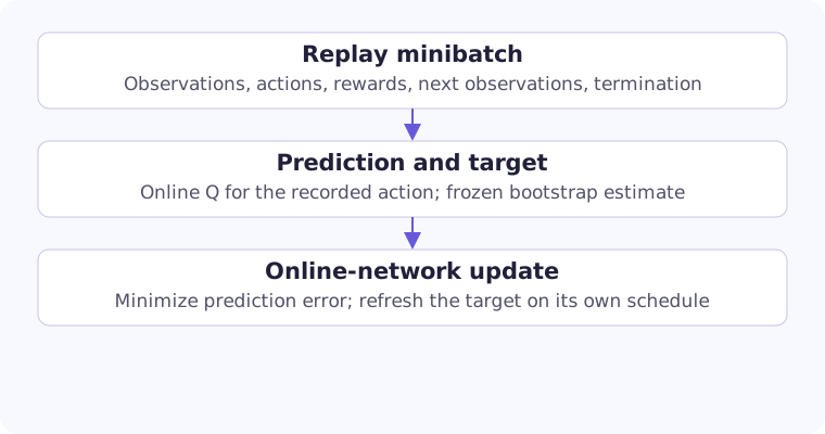
For a discrete action set, the network returns a vector \([Q_\theta(s,0),\ldots,Q_\theta(s,A-1)]\). The environment supplies a transition \((s,a,r,s^{\prime})\). We train the entry for the action actually taken, including exploratory actions; it need not have been the network’s favourite.
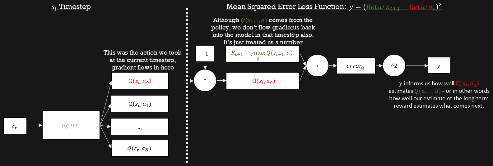
Let \(d\) indicate a true terminal transition. With a target network whose parameters are \(\bar\theta\), the target and squared loss are $$y=r+\gamma(1-d)\max_{a^{\prime}}Q_{\bar\theta}(s^{\prime},a^{\prime}),\qquad L=(Q_\theta(s,a)-y)^2.$$ During this update, \(y\) is treated as a constant. This is a semi-gradient update: we differentiate the current prediction, not the bootstrapped target.
Selecting one output for the loss does not isolate every effect of learning to that action. The shared hidden layers can change other outputs and predictions at other states. This is the generalization—and interference—we introduced in the function-approximation post.
The original loss diagram separates the recorded action’s prediction from the next-state target. Read its Return labels as shorthand for the current Q prediction and bootstrapped target, not complete Monte Carlo returns. The target contributes a number to the error; gradients enter through the selected current output.
The semi-gradient makes the connection to Q-learning explicit
For a minibatch of \(B\) transitions, use \(L(\theta)=\frac1{2B}\sum_i(Q_\theta(s_i,a_i)-y_i)^2\). With each target held fixed, $$\nabla_\theta L=\frac1B\sum_i(Q_\theta(s_i,a_i)-y_i)\nabla_\theta Q_\theta(s_i,a_i).$$ Gradient descent moves the prediction toward its target along directions the network can represent. If each prediction had its own independent scalar parameter and the batch contained one transition, this would be exactly the tabular Q-learning update.
The network generally cannot satisfy every sampled target independently because parameters are shared. Nor are the targets ground-truth labels: they are one reward plus an estimated greedy continuation. Function approximation, bootstrapping, and off-policy sampling can interact to destabilize learning. The contraction proof for an exact tabular Bellman operator does not directly transfer to a neural-network optimizer operating on replayed samples.
Experience replay changes which data we learn from
The naive course example updates immediately from each new transition. Consecutive observations are strongly related, and a short sequence can dominate the current updates. Useful experiences are also discarded after one use.
A replay buffer retains transitions. To learn, we sample a minibatch from that buffer and construct fresh targets using the current networks. Store observations, actions, rewards, next observations, and termination flags, rather than old Q-values. Sampling reduces temporal correlation and permits repeated use of an interaction; it does not make a finite, changing buffer perfectly independent or representative.
Q-learning is off-policy: the maximizing action in the target may differ from the action selected by the behaviour policy. This makes replay from older behaviour policies natural here. It does not imply that an arbitrary policy-gradient update can reuse old trajectories without correction.
The buffer defines a concrete training distribution
At a fixed instant, a buffer containing \(M\) transitions defines the empirical loss $$L_{\mathcal D}(\theta)=\frac1M\sum_{i=1}^M\frac12\big(Q_\theta(s_i,a_i)-y_i\big)^2.$$ Uniform minibatch sampling estimates its semi-gradient. It need not sample states in the proportions that the final greedy policy will encounter them. A rare state remains rare in the training loss unless the collection or sampling scheme makes it more prominent.
The ratio of optimizer steps to environment steps controls how heavily we reuse this finite experience. Too few updates can leave useful data underused; many updates can fit a narrow, stale buffer repeatedly. Replay does not create new information about actions never tried. Its off-policy use is justified at the transition level because, in a stationary MDP, the conditional outcome distribution for a recorded \((s,a)\) does not depend on which past policy selected it. Approximation error outside that coverage remains a problem.
A slower target is a separate mechanism
If both sides of the loss use the same rapidly changing network, each parameter update also moves the training target. DQN uses a separate target copy. Initialize it from the online network, update only the online network by gradient descent, and periodically copy its weights into the target network. A soft update is another option, but the choice and cadence should be stated.
Replay controls the distribution of training examples. The target network controls how quickly the bootstrap estimates change. Neither guarantees convergence for nonlinear off-policy learning. Track episodic return as well as the optimization loss.
Target updates turn moving targets into slower regression problems
A hard target update sets \(\bar\theta\leftarrow\theta\) every \(C\) learning steps. Between copies, replay targets depend on a fixed target network, although new transitions can still enter the buffer. A soft update instead uses $$\bar\theta\leftarrow(1-\tau)\bar\theta+\tau\theta,\qquad0<\tau\le1.$$ This exponentially averages successive online parameters. It is not generally identical to averaging their output predictions, since a neural network is nonlinear in its parameters.
Holding a target network fixed resembles a sequence of regression problems: fit a current approximation to one Bellman backup of an older approximation, then refresh the target. A very fast refresh recovers more of the moving-target problem; a very slow refresh propagates improved values slowly. Both mechanisms address optimization behavior, and neither proves that the learned action values equal \(Q^*\).
Double DQN separates selection from evaluation
A maximum tends to select positive estimation errors. Double DQN first selects an action with the online network, then evaluates that action using the target network: $$a^*=\arg\max_a Q_\theta(s^{\prime},a),\qquad y=r+\gamma(1-d)Q_{\bar\theta}(s^{\prime},a^*).$$ Simply having two network copies is not the distinguishing step; ordinary DQN already has a target network.
| At the next state | Action 0 | Action 1 |
|---|---|---|
| Online estimates | 8 | 7 |
| Target estimates | 4 | 6 |
For reward 1 and discount 0.9, ordinary DQN uses the target maximum 6 and produces a target of 6.4. Double DQN selects action 0 using the online estimates, evaluates it as 4, and produces 4.6. This is a deliberately constructed example of the difference, not evidence that either target is closer to the unknown true value.
Double Q-learning: van Hasselt, Guez, and Silver
Why maximizing noisy estimates produces a directional error
Suppose the estimates at a state are \(\hat q_a=q_a+e_a\), with zero-mean errors for each action. Because the maximum is convex, $$\mathbb E[\max_a\hat q_a]\ge\max_a\mathbb E[\hat q_a]=\max_aq_a.$$ Zero-mean individual errors do not imply a zero-mean error after selecting the largest estimate.
For a small exact example, let two actions both truly be worth zero, and let their independent errors be +1 or −1 with equal probability. Their maximum is +1 in three of four cases and −1 in one, so its expectation is 0.5. Evaluating the selected action with an independent zero-mean estimator removes that positive bias in this equal-value example. With unequal true values, selection can still choose the wrong action. Double DQN's online and target estimates are also correlated, so its construction mitigates a source of error without guaranteeing unbiased or correct targets.
The minibatch update in PyTorch
This function expects two matching networks, an optimizer for online only, and a replay minibatch. States have shape [B, observation_dimensions]; actions are integer indices of shape [B]. Rewards and terminated flags also have shape [B]. It implements Double DQN; replacing the two selection/evaluation lines with target(next_states).max(dim=1).values gives the ordinary DQN target.
import torch
from torch.nn import functional as F

def double_dqn_step(online, target, optimizer, states, actions,
                    rewards, next_states, terminated, gamma=0.99):
    predicted = online(states).gather(1, actions[:, None]).squeeze(1)
    with torch.no_grad():
        selected = online(next_states).argmax(dim=1, keepdim=True)
        next_q = target(next_states).gather(1, selected).squeeze(1)
        y = rewards + gamma * (~terminated.bool()).float() * next_q
    loss = F.mse_loss(predicted, y)
    optimizer.zero_grad()
    loss.backward()
    optimizer.step()
    return loss.item()

# Initialize once, then repeat at the chosen target-update interval:
# target.load_state_dict(online.state_dict())
The surrounding collector must distinguish termination from truncation. Both usually end the current rollout, but an external time-limit truncation can still bootstrap from the final observation. A true terminal state cannot. This distinction depends on how the task defines its horizon; a time limit that belongs to the task is part of the termination semantics.
Gymnasium: handling time limits
The snippet is an update kernel, not a complete CartPole experiment. The collector, exploration schedule, replay capacity, warm-up period, and target-copy schedule remain explicit parts of a full implementation.
Squared error versus a bounded influence from large residuals
Let \(e=Q_\theta(s,a)-y\). Squared loss has derivative proportional to \(e\), so unusually large target errors can dominate a minibatch. A Huber loss with threshold \(\kappa>0\) is $$\ell_\kappa(e)=\begin{cases}\tfrac12e^2,&|e|\le\kappa,\\\kappa(|e|-\tfrac12\kappa),&|e|>\kappa.\end{cases}$$ Its derivative is \(\operatorname{clip}(e,-\kappa,\kappa)\). This bounds the residual's multiplier on the prediction gradient, but does not necessarily bound the whole parameter gradient when the network Jacobian is large.
The displayed kernel deliberately uses mean squared error, so a Huber version would be an explicit loss change. Gradient clipping is yet another mechanism: it acts on parameter gradients after differentiation. Keeping the target construction, regression loss, and optimizer controls distinct makes an experiment interpretable.
Dueling changes the representation
A dueling network splits its final representation into a scalar stream and an action-dependent stream: $$Q(s,a)=V(s)+A(s,a)-\frac{1}{|\mathcal A|}\sum_b A(s,b).$$ Subtracting the mean fixes the otherwise ambiguous decomposition: adding a constant to every advantage and subtracting it from the value would leave Q unchanged.
This structure lets learning share information about how favourable a state is even when many actions have similar values. Its mean-centred advantage stream should not automatically be equated with the exact policy-weighted advantage from policy-gradient theory. Dueling is an architectural choice; Double DQN is a target construction. They can be combined.
Dueling networks: Wang and colleagues
What the two dueling streams learn to identify
For \(K\) actions, denote the raw advantage outputs by \(A_1,\ldots,A_K\). With mean subtraction, $$\frac{\partial Q(s,a)}{\partial A_j}=\mathbf1\{j=a\}-\frac1K,\qquad\frac{\partial Q(s,a)}{\partial V}=1.$$ A loss on one chosen action sends a full signal to the common value stream and a centered signal across the advantage outputs. Averaging Q over all actions gives the value stream exactly, \(K^{-1}\sum_aQ(s,a)=V(s)\).
This is an arithmetic average over available actions, not a policy-weighted expectation unless the policy is uniform. The network's raw advantage logits themselves still admit a shared constant shift; centering removes that shift from Q and fixes the effective zero-mean advantage used in the decomposition. These details distinguish an architectural factorization from the advantage function used to weight policy gradients.
A course experiment worth comparing
Start from the same observation network and discrete-action task, then compare online-only updates, replay with a target network, and Double DQN. Keep interaction budgets and evaluation procedures comparable. Report returns across several seeds and record environment steps separately from gradient steps; more replay updates do not mean more environment experience.
Plotting only the loss would miss the central question. A model may closely fit inaccurate bootstrap targets while behaving poorly. Evaluate a fixed greedy policy separately from exploratory training, and inspect Q-value scale alongside reward. The course’s progression is most informative when each comparison changes one mechanism at a time.
Next: learn action probabilities with REINFORCE
Adapted from my reinforcement learning course: module 06, slides 7–22; deepqlearning_naive.py, replay_memory.py, agents.py, and deep_q_network.py. The worked examples in this post are teaching examples, not benchmark results.