Our CartPole example made continuous observations manageable by assigning them to bins. That let us keep a Q-table, but the boundaries and resolution were choices we imposed on the problem. What happens when there are too many variables to build a useful grid? This is where the course turns from tables to function approximation.
When a table becomes the bottleneck
If each of \(d\) observation dimensions has \(b\) bins and there are \(A\) actions, a dense Q-table contains \(b^d A\) entries. Ten bins along four coordinates and two actions require 20,000 entries. With eight coordinates and four actions, the same resolution requires 400 million. More memory alone does not provide the experience needed to estimate every entry.
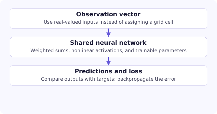
Instead, write \(Q_\theta(s,a)\): a function whose parameters \(\theta\) are shared across inputs. A transition at one state changes the parameters, potentially changing estimates at nearby states too. This sharing makes generalization possible, but it also makes interference possible. Improving one prediction can worsen another.
Continuous observations and continuous actions are separate issues. A network can accept a real-valued observation vector while still returning one Q-value for each of a small number of discrete actions. We will use exactly that arrangement in DQN.
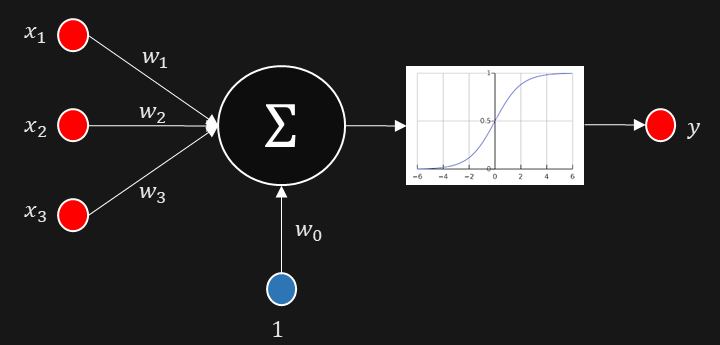
The original neuron diagram makes the weighted sum concrete: each input arrives along a weighted connection, while the constant input supplies the bias. The activation then transforms the combined signal.
From independent table entries to shared features
A useful intermediate model is linear function approximation, \(Q_w(s,a)=w^\top\phi(s,a)\), where \(\phi\) is a chosen feature vector. A table is a special case: give every state-action pair its own one-hot feature. Then only one weight contributes to a prediction. With overlapping features, several observations depend on the same weights, so learning from one observation can affect the others. A neural network goes further by learning the intermediate features as well as their final combination.
To make learning precise, first imagine a dataset of fixed regression targets \(y_i\). Choose parameters by minimizing $$L(\theta)=\frac1{2N}\sum_{i=1}^N\big(Q_\theta(s_i,a_i)-y_i\big)^2.$$ The squared error penalizes large residuals, and the factor one-half simplifies the derivative. For a single linear prediction, $$\nabla_w\frac12(Q_w-y)^2=(Q_w-y)\phi(s,a),\qquad w\leftarrow w+\eta(y-Q_w)\phi(s,a).$$ With one-hot features this changes just the corresponding table entry. The tabular update and the learned predictor are now visibly two versions of the same error-correction idea.
The data distribution matters as much as the model class. More generally we minimize an expectation under a sampling distribution \(\nu(s,a)\). States seldom represented in that distribution exert little influence on the loss. Generalization to those states comes from assumptions imposed by the representation; a low average error on familiar observations does not certify correct values elsewhere.
What a neuron actually computes
A neuron first forms a weighted sum and then applies an activation: $$z=w^\top x+b,\qquad h=\sigma(z).$$ The weights control how inputs contribute; the bias shifts the response. Without an activation, this is an affine function. Chaining affine layers still produces an affine function, however many layers we add.
ReLU, \(\sigma(z)=\max(0,z)\), allows a network to combine different linear regions. Depth composes these transformations; it does not assign a fixed polynomial degree to the model. A two-layer network is not automatically a quadratic function.
The output activation depends on what the numbers mean. A Q-network usually has unrestricted real-valued outputs because returns can be negative or larger than one. A categorical policy uses logits that define action probabilities. A digit classifier may look architecturally similar, but its outputs and training targets answer a different question.
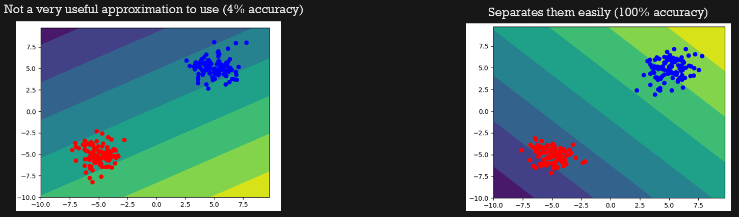
These two examples from the slides use the same simple model class with different parameters. The coloured response surfaces separate the synthetic clusters very differently. The displayed accuracies describe these teaching examples, not performance on a held-out RL task.
Writing an entire network as a composition
Let \(h^{(0)}=x\). A network with \(L\) layers computes $$z^{(\ell)}=W^{(\ell)}h^{(\ell-1)}+b^{(\ell)},\qquad h^{(\ell)}=\sigma_\ell(z^{(\ell)}),\quad\ell=1,\ldots,L.$$ If layer \(\ell\) has \(n_\ell\) units, its weight matrix has shape \(n_\ell\times n_{\ell-1}\) and its bias has \(n_\ell\) entries. For Q regression the final activation is commonly the identity, permitting arbitrary signed values.
Why introduce nonlinearity? Two affine layers without it collapse to $$W_2(W_1x+b_1)+b_2=(W_2W_1)x+(W_2b_1+b_2).$$ The extra parameters do not create a richer family of input-output functions. ReLU instead changes which units are active as the input changes. Tanh gives bounded hidden activations, but its derivative \(1-\tanh^2z\) becomes small at large magnitudes. This affects gradient propagation; the activation is part of both the representation and the optimization problem.
A gradient-descent example we can solve by hand
The course uses \(f(x)=5x^2-4x+10\). Its derivative is \(10x-4\), so the minimum is at \(x=0.4\). Gradient descent takes a step opposite the derivative: $$x_{k+1}=x_k-\eta f^{\prime}(x_k).$$ With \(x_0=10\) and \(\eta=0.05\), the first exact-gradient update gives \(5.2\). Subsequent iterates are \(2.8,1.6,1.0,0.7\).
We can also estimate the slope from function evaluations: $$f^{\prime}(x)\approx\frac{f(x+h)-f(x)}{h}.$$ This forward difference is approximate. For this quadratic it equals \(10x-4+5h\), so using \(h=0.01\) converges toward 0.395 rather than exactly 0.4. That small discrepancy is explained by the method, not random training noise.
def f(x):
    return 5*x*x - 4*x + 10

x, h, learning_rate = 10.0, 0.01, 0.05
for _ in range(20):
    slope = (f(x + h) - f(x)) / h
    x -= learning_rate * slope
print(round(x, 6))  # 0.395009
This example runs with Python alone. Try a smaller step size for the optimizer, then a different finite-difference spacing. These are different parameters: one controls how far we move, the other controls how we estimate the slope. Making the spacing extremely small eventually introduces floating-point cancellation.
Why the learning rate can make the same gradient fail
For the quadratic above, subtract the minimizer from both sides of the update: $$x_{k+1}-0.4=(1-10\eta)(x_k-0.4).$$ Convergence requires \(|1-10\eta|<1\), or \(0<\eta<0.2\). A step of 0.05 halves the error each iteration; a step of 0.15 alternates around the minimum while shrinking it; 0.2 oscillates without shrinking. A correct derivative does not rescue an unsuitable step size.
For a smooth multidimensional loss, a first-order expansion gives $$L(\theta+\Delta)\approx L(\theta)+\nabla L(\theta)^\top\Delta.$$ Taking \(\Delta=-\eta\nabla L\) predicts a decrease of \(\eta\|\nabla L\|^2\) locally. Curvature limits how far that approximation remains useful. Neural-network losses are generally nonconvex, so the simple quadratic calculation illustrates local step-size behavior without establishing convergence to a global optimum.
Backpropagation is the chain rule, reused
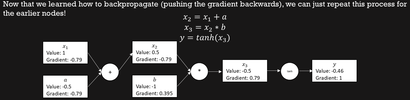
Now consider the course’s small computational graph: $$u=x+a,\quad v=ub,\quad y=\tanh(v).$$ At \(x=1,a=-0.5,b=-1\), we get \(u=0.5,v=-0.5,y\approx-0.4621\). Working backwards gives $$\frac{\partial y}{\partial a}=(1-y^2)b\approx-0.7864,\qquad \frac{\partial y}{\partial b}=(1-y^2)u\approx0.3932.$$
Each operation supplies a local derivative. Multiplying it by the gradient arriving from the output gives the gradient for an earlier node. Intermediate results are reused instead of perturbing every weight and running the entire network again. Automatic differentiation records these operations; an optimizer subsequently uses their gradients to change parameters.
Only trainable parameters are updated. Calculating a derivative with respect to an input or intermediate value does not mean the training loop should alter that observation. And in a real predictor, we usually differentiate a loss built from the output, rather than simply trying to make the output smaller.
The computational graph below carries the forward values and backward gradients at the same time. The slides call the intermediate values x₂ and x₃; they correspond to u and v in the equations above. Follow the chain from tanh through multiplication to addition to recover the two parameter derivatives.
Backpropagating a loss through every layer
The small tanh graph differentiated its output. For training, begin instead with a scalar loss \(L\), such as half the squared output error, and define \(\delta^{(\ell)}=\partial L/\partial z^{(\ell)}\). For an identity output layer with squared error, \(\delta^{(L)}=h^{(L)}-y\). Hidden-layer errors satisfy $$\delta^{(\ell)}=\big((W^{(\ell+1)})^\top\delta^{(\ell+1)}\big)\odot\sigma_\ell'(z^{(\ell)}).$$ The symbol \(\odot\) means elementwise multiplication: first accumulate the downstream influence, then multiply by each unit's local derivative.
The parameter gradients follow directly: $$\frac{\partial L}{\partial W^{(\ell)}}=\delta^{(\ell)}(h^{(\ell-1)})^\top,\qquad\frac{\partial L}{\partial b^{(\ell)}}=\delta^{(\ell)}.$$ A minibatch averages these contributions. Repeated multiplication by small derivatives can weaken the signal reaching early layers; large matrix factors can amplify it. This is the mathematical reason activation choice, input scale, and initialization can materially affect learning, even when the network has enough parameters to express a useful function.
A small PyTorch training step
The course’s MNIST example introduces tensors, batches, and train/validation/test splits. For the RL bridge, the same mechanics can be shown with four observations and two action-value outputs. This illustrative batch uses made-up regression targets; it is not an agent training run.
import torch
from torch import nn

torch.manual_seed(0)
model = nn.Sequential(nn.Linear(4, 32), nn.ReLU(), nn.Linear(32, 2))
optimizer = torch.optim.Adam(model.parameters(), lr=1e-3)
states = torch.tensor([[0.0, 0.2, -0.1, 0.3],
                       [0.1, 0.0, 0.2, -0.2]])
targets = torch.tensor([[1.0, 2.0], [0.5, -1.0]])

prediction = model(states)  # [batch=2, actions=2]
loss = nn.functional.mse_loss(prediction, targets)
optimizer.zero_grad()
loss.backward()
optimizer.step()
The model has 226 parameters: 32 × (4 + 1) in the first layer and 2 × (32 + 1) in the output layer. Its parameter count does not grow when a new observation arrives. Its ability to represent and learn useful values is still limited by architecture, data coverage, and optimization.
zero_grad clears gradients accumulated by earlier backward passes. backward computes derivatives of this loss. step performs the parameter update. These three operations are related, but none substitutes for the others.
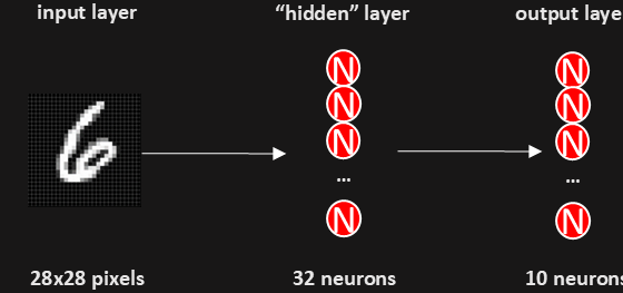
The course’s digit-recognition diagram shows how a fixed input dimension feeds a hidden layer and a task-specific output layer. Here the ten outputs describe digit classes; in the smaller code example above, the two outputs instead represent action-value predictions.
A minibatch estimates a gradient, not a new objective
For \(B\) independently sampled training examples, the average gradient is an unbiased estimate of the dataset-average gradient, conditional on fixed parameters and a fixed dataset. Batching reduces sampling noise and makes matrix operations efficient. Correlated or changing RL data complicate that idealized picture, which is why the next post examines replay explicitly.
The code's mean-squared loss averages over both batch entries and the two action outputs; it omits the one-half used in the derivation. These conventions rescale gradients without changing the minimizer for fixed targets. In actual DQN, only the recorded action has a transition target, so the loss selects that action's output rather than inventing targets for every action.
The optimizer shown is Adam. For gradient \(g_k\), it keeps moving moments \(m_k=\beta_1m_{k-1}+(1-\beta_1)g_k\) and \(v_k=\beta_2v_{k-1}+(1-\beta_2)g_k^2\). After bias corrections \(\hat m_k=m_k/(1-\beta_1^k)\) and \(\hat v_k=v_k/(1-\beta_2^k)\), its elementwise update is $$\theta_{k+1}=\theta_k-\eta\frac{\hat m_k}{\sqrt{\hat v_k}+\epsilon_{\mathrm{num}}}.$$ The small denominator constant prevents numerical division problems; it is unrelated to epsilon-greedy exploration. Adam changes how gradients are used, not how backpropagation computes them.
What changes when the target is a return?
In supervised regression, the supplied targets can remain fixed while the model changes. In deep reinforcement learning, the target often contains another value prediction. The learner is then changing the estimates it will use to supervise future updates. A low training loss can mean agreement between estimates without proving that the resulting policy earns a high return.
For a return target, Monte Carlo regression uses \(y=G_t\). A Q-learning target uses \(y=r+\gamma(1-d)\max_bQ_{\bar\theta}(s',b)\). Holding that target fixed gives \(\Delta\theta=\eta(y-Q_\theta)\nabla_\theta Q_\theta\). If the target were differentiated too, the squared-loss derivative would instead contain \(\nabla_\theta Q_\theta-\nabla_\theta y\). That is a different algorithm. The useful transition is therefore larger than replacing a table lookup with a forward pass. We must specify what the output represents, where its target comes from, and which computations receive gradients. The next post uses the Bellman target to make those decisions explicit.
Adapted from my reinforcement learning course: module 05, slides 2–5, 7–19, 20–37; finite_differences.py, finite_difference_network.py, and pytorch_introduction.py. The worked examples in this post are teaching examples, not benchmark results.