RL interaction loop
At time \(t\), the agent chooses an action \(a_t\) from a policy \(\pi\), the environment transitions, and the agent receives a reward \(R_t\). This is the basic feedback loop that everything else builds on, brute force search or other strategies rely on this Markov Decision Process (MDP) structure. We can describe how an intelligent agent may interact with its environment over discrete time steps with the below image.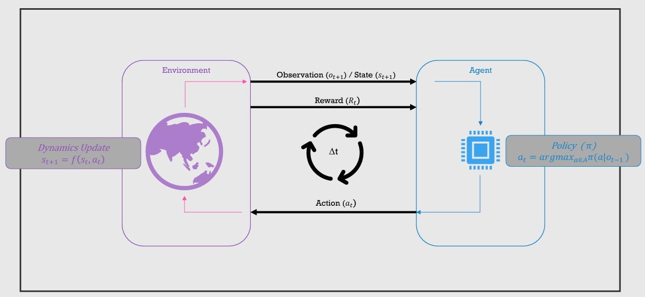 From this starting point, we can formalize the agent's decision-making process and the environment's response as follows: $$ A_t\sim\pi(\cdot\mid S_t),\qquad (S_{t+1},R_{t+1})\sim p(\cdot,\cdot\mid S_t,A_t). $$ For deterministic dynamics this simplifies to \(s_{t+1}=f(s_t,a_t)\). Exact tabular DP requires transition probabilities and expected rewards; a simulator that only supplies samples supports sampled backups instead.
The Bellman Equation: value is “reward now + value later”
For a deterministic transition under a fixed deterministic policy, a compact recursion is: $$ V(s_i) = R_i + \gamma V(s_{i+1}). $$ This is a simple way to internalize the core idea: the value of being in a state is the immediate reward plus a discounted version of what comes next. The “full” Bellman expectation equation makes the probabilities explicit: $$ V^\pi(s)=\sum_a \pi(a\mid s)\sum_{s',r} p(s',r\mid s,a)\left[r + \gamma V^\pi(s')\right]. $$ This full Bellman equation makes it more clear how the value for a state is computed. In its original format, as displayed above, it relies on knowing the outcomes you would get from taking all possible actions in that state, weighted by the policy's action probabilities and the environment's transition probabilities. This means that to have a true value estimate, you'd need to know the result of going down all forks in the road.Brute force search for \(V^\pi(s)\)
Brute force mindset. If you want a policy that does the best actions over the next \(N\) steps: just look ahead over all possibilities for those \(N\) steps and choose the best one. Even the one-step picture is intuitive: you start at a state, branch over actions, branch to the next states, and back up the best outcome to define \(V(s)\).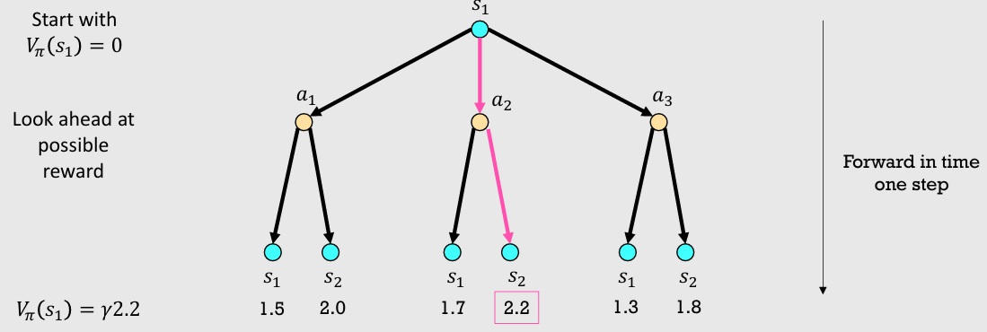 Where it breaks. As soon as you look ahead more than one step, the tree balloons. Each extra timestep multiplies the number of future branches you must consider.
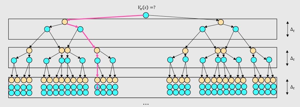 The important scaling facts are: - it scales multiplicatively with the number of actions,
- it scales multiplicatively with the number of states, and
- it scales exponentially with how many timesteps you look ahead. To brute-force a Bellman-style lookahead, you typically need: 1) a dynamical model that predicts \(s'\) and reward \(r\);
2) the Markov property (next state depends only on current state and action);
3) enough compute to actually search the tree. If we denote: - \(N\): planning horizon (timesteps looked ahead),
- \(n_x\): number of states (or discretized states),
- \(n_u\): number of actions, then the brute-force optimization cost is often summarized as: $$ \mathcal{O}\big(n_x (n_x n_u)^N\big). $$ A toy number from the lecture story: look ahead 10 timepoints with 10 states and 3 actions. That gives \(10 \cdot 30^{10} \approx 5.9\times 10^{15}\) possibilities. This is already dead-on-arrival.
This is the core motivation: “true value estimation” by explicitly enumerating futures becomes infeasible extremely quickly. So the real question is: can we keep the Bellman logic without paying exponential time in \(N\)?
The repeated subproblem hidden inside the search tree
Many branches reach the same state with the same amount of time remaining. A Markov model says those branches then share the same continuation problem. For a finite horizon of \(H\) decisions, define \(V_h^*(s)\) as the best expected return with \(h\) decisions left. With terminal payoff \(g\), backward induction is $$V_0^*(s)=g(s),\qquad V_h^*(s)=\max_a\sum_{s',r}p(s',r\mid s,a)\big[r+\gamma V_{h-1}^*(s')\big].$$ Store one answer per state and remaining horizon instead of recalculating it for every history that arrives there.
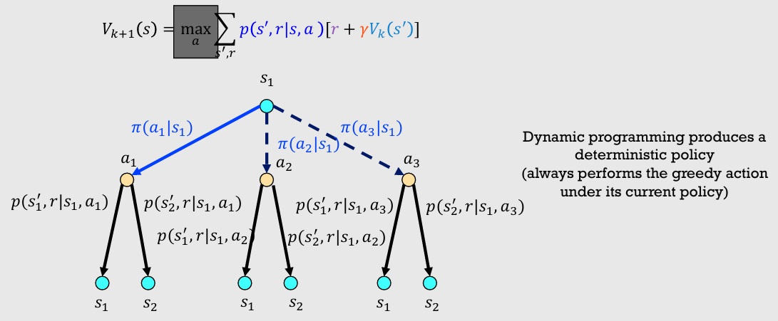
The maximum chooses an action; the expectation averages over the environment's response. Choosing the best possible successor state would let the agent control randomness that actually belongs to the environment. For policy evaluation, replace the maximum with an average under \(\pi\). These are different backups even if the drawings of their search trees look similar.
With \(n_x\) states, \(n_u\) actions, and dense transitions, one full sweep costs \(O(n_x^2n_u)\). A finite-horizon solution takes \(O(Hn_x^2n_u)\), linear in the horizon rather than exponential. If every action has at most \(b\) possible successors, the cost is \(O(Hn_xn_ub)\). This calculation excludes the cost of obtaining the model and still requires storing or accessing its transitions.
Dynamic programming: break the problem into subproblems
Dynamic programming changes the computation, not the goal. Instead of searching all length-\(N\) futures, DP repeatedly solves a simpler subproblem: “Given my current estimate of the future, what is the best one-step backup for each state?” Then it repeats those backups until the values stabilize. This is the first major pattern you see in reinforcement learning: alternate between improving values and improving the policy.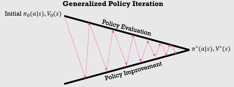
This alternating pattern is called generalized policy iteration (GPI): - Policy evaluation: update \(V\) for a fixed \(\pi\).
- Policy improvement: update \(\pi\) to be greedier w.r.t. the latest \(V\).
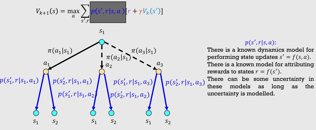
DP is “early RL” largely because it is clean and principled under strong assumptions: the transition probabilities and expected rewards are known, and you can enumerate states/actions (tabular setting). A simulator that only samples transitions does not directly supply exact expectation backups.
Policy evaluation (Bellman expectation backup)
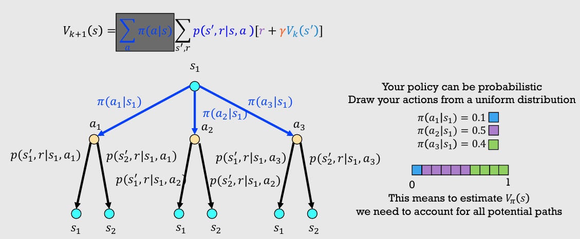
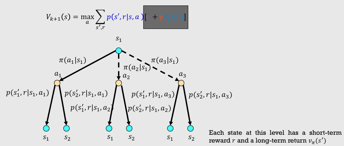
Policy Evaluation. If the policy \(\pi\) is fixed, we update value estimates by applying a Bellman backup: $$ V_{k+1}(s)=\sum_a \pi(a\mid s)\sum_{s',r} p(s',r\mid s,a)\left[r + \gamma V_k(s')\right]. $$ Intuition: you’re averaging over all actions the policy might take and all outcomes the environment might produce. This is where knowing the model matters: DP is literally computing the expectation.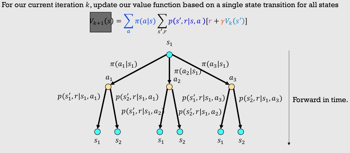
A numerical evaluation sweep and its fixed point
Consider a policy that stays in a single nonterminal state with probability 0.8 and otherwise terminates. Suppose every step from that state pays 1 and \(\gamma=0.9\). Its evaluation equation is $$V^\pi(s)=1+0.72V^\pi(s),\qquad V^\pi(s)=\frac1{1-0.72}\approx3.5714.$$ Starting from zero, synchronous sweeps give 1, 1.72, and 2.2384. Each sweep propagates another layer of possible future reward; it is not another physical trial of the system.
For a finite model, collect the policy-weighted rewards and transitions into \(R^\pi\) and \(P^\pi\). Solving \((I-\gamma P^\pi)V=R^\pi\) evaluates the policy directly. Iterative evaluation trades an exact linear solve for repeated cheaper backups. A synchronous sweep reads exclusively from the previous value table; an in-place sweep can use values already updated during the same sweep. Under discounted tabular assumptions, both can converge, but their intermediate numbers and stopping diagnostics differ.
Policy Improvement
Once you have a decent estimate of value, improving the policy becomes the straightforward step: for each state, pick the action with the best expected one-step outcome plus downstream value. $$ \pi_k(s)\in\arg\max_{a\in\mathcal A}\sum_{s',r}p(s',r\mid s,a)\left[r+\gamma V_k(s')\right]. $$ Narratively: policy evaluation answers “how good is each state under my current behavior,” and policy improvement answers “given that, what should I do next time I’m in this state?”Why a greedy improvement cannot make an exact policy worse
Let \(\pi'\) choose actions maximizing the one-step return computed from the exact \(V^\pi\). Then $$T^{\pi'}V^\pi\ge T^\pi V^\pi=V^\pi.$$ Bellman operators preserve inequalities because their transition weights are nonnegative. Repeatedly applying \(T^{\pi'}\) therefore produces a nondecreasing sequence beginning at \(V^\pi\), and its limit is \(V^{\pi'}\). Thus \(V^{\pi'}(s)\ge V^\pi(s)\) for every state.
This explains the evaluation–improvement loop rather than merely naming it. Improvement need not be strict in every state, and ties between equally good actions are possible. Consistent tie-breaking prevents a policy-iteration implementation from switching forever between equivalent choices. With approximate evaluation, the exact monotonicity argument no longer applies automatically; action rankings can be wrong when their gaps are smaller than the value-estimation errors.
Stopping Criterion
The algorithmic picture from the lecture is: initialize values (often via terminal costs), repeat backups and greedy improvements, stop when the values stabilize.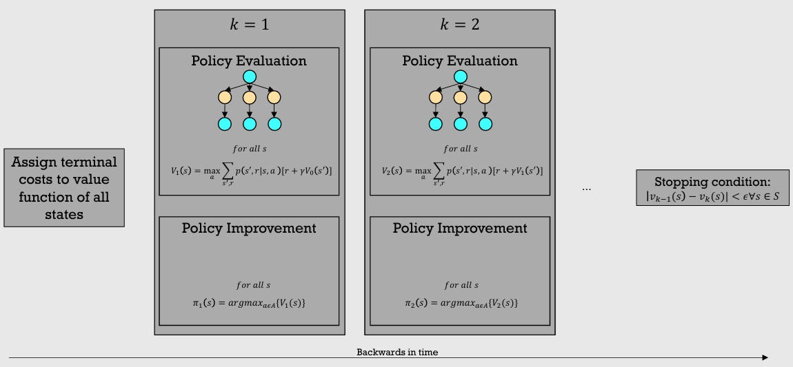 A typical convergence criterion is: $$ |V_k(s) - V_{k-1}(s)| < \varepsilon \qquad \forall s\in\mathcal{S}. $$ The key computational win vs brute force: DP avoids exponential dependence on horizon \(N\) by reusing “value of subproblems.” It can still be expensive in the number of states (curse of dimensionality), but it’s no longer hopeless for small tabular models.
What a stopping rule actually certifies
For exact synchronous value iteration, the change \(\|V_{k+1}-V_k\|_\infty\) is the Bellman residual of \(V_k\). A residual below \(\varepsilon\) bounds its value error by \(\varepsilon/(1-\gamma)\). A small fraction of changed policy entries is a different diagnostic: it says the selected actions have mostly stabilized, not that the value residual is small.
If an estimate \(V\) is within \(e\) of \(V^*\) in sup norm, its greedy policy satisfies $$\|V^*-V^{\pi_V}\|_\infty\le\frac{2\gamma e}{1-\gamma}.$$ To see the factor two, compare both the optimal action and the action chosen using \(V\): each one-step continuation estimate can be wrong by \(\gamma e\). Repeated future decisions contribute the remaining geometric factor. This is a worst-case discounted finite-model guarantee, not a bound on a discretized controller's physical tracking error.
Example: Inverted Pendulum
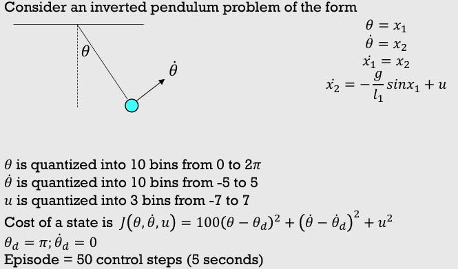
You can consult the code here:
rl_3_dynamicprogramming.py
Connecting the pendulum to a well-defined control objective
For the illustrated pendulum, let \(s=(\theta,\omega)\), with angle measured from upright. Using angular acceleration input \(u\), a simple model is $$\dot\theta=\omega,\qquad\dot\omega=\frac{g}{\ell}\sin\theta+u.$$ If the control were torque instead, its contribution would need the appropriate inertia factor. An Euler step of duration \(\Delta t\) gives \(\theta'=\theta+\Delta t\,\omega\) and \(\omega'=\omega+\Delta t[(g/\ell)\sin\theta+u]\).
To formulate a standard discounted controller, choose a fixed stage cost such as \(c(s,u)=q_\theta\operatorname{wrap}(\theta)^2+q_\omega\omega^2+\lambda u^2\), with nonnegative weights. The cost-to-go backup is $$C_{k+1}(s)=\min_u\big[c(s,u)+\gamma C_k(f_{\Delta t}(s,u))\big].$$ This is the reward formulation with \(r=-c\). Interpolation or nearest-bin lookup is needed when the predicted successor falls between grid points. Finer grids reduce some representation errors but increase the number of values and model evaluations.
The linked legacy demonstration uses a different accumulated-cost update and a policy-change stopping rule. Its animation illustrates the controller lookup, but does not establish convergence of the discounted backup derived here. It also retains a simulation integrator that reads the stored acceleration in the velocity slot; its physical trajectory should not be used to validate these equations. Separating the mathematical objective, numerical transition model, and stopping rule is essential before interpreting a simulation as evidence about control performance.
Quiz questions
Q: Brute force scales exponentially with what?Q: Dynamic programming scales exponentially with what?
Q: What do we need to use dynamic programming?
Q: Dynamic programming is an application of GPI.
Q: What is the purpose of policy evaluation?
Q: What is the purpose of policy improvement?