- Competitive games such as chess, backgammon, or Go.
- Complex locomotion and driving tasks where dynamics are hard to write down exactly.
Monte Carlo intuition (π from random samples).
MC approximates a value by successive random samples. To estimate \(\pi\):- Area of a square: \(A_{\text{square}} = l \cdot w\).
- Area of a circle: \(A_{\text{circle}} = \pi r^2\).
- Set \(r = 0.5\), \(l = w = 1.0\). Then \(\frac{A_{\text{circle}}}{A_{\text{square}}} = \pi/4\), so \(\pi = 4 \cdot \frac{A_{\text{circle}}}{A_{\text{square}}}\).
A sample average is an estimator of an expectation
Let \(I_i\) indicate whether the \(i\)-th uniformly sampled point lies inside the circle. Then \(I_i\) is Bernoulli with probability \(\pi/4\), and $$\hat\pi_N=\frac4N\sum_{i=1}^N I_i,\qquad \mathbb E[\hat\pi_N]=\pi,\qquad\operatorname{Var}(\hat\pi_N)=\frac{16}{N}\frac\pi4\left(1-\frac\pi4\right).$$ The numerical constant \(\pi\) here is unrelated to the policy symbol used in RL. Increasing the number of independent samples reduces standard error at rate \(N^{-1/2}\).
For policy evaluation, replace the circle indicator with a trajectory return conditioned on visiting a particular state-action pair. The model is sampled by interacting with the environment rather than enumerated during a Bellman backup. We still need a specified policy, enough visits to the pair of interest, and returns with suitable finite moments. No model requirement does not mean no statistical assumptions.
Monte Carlo policy evaluation (for \(Q^\pi\)).
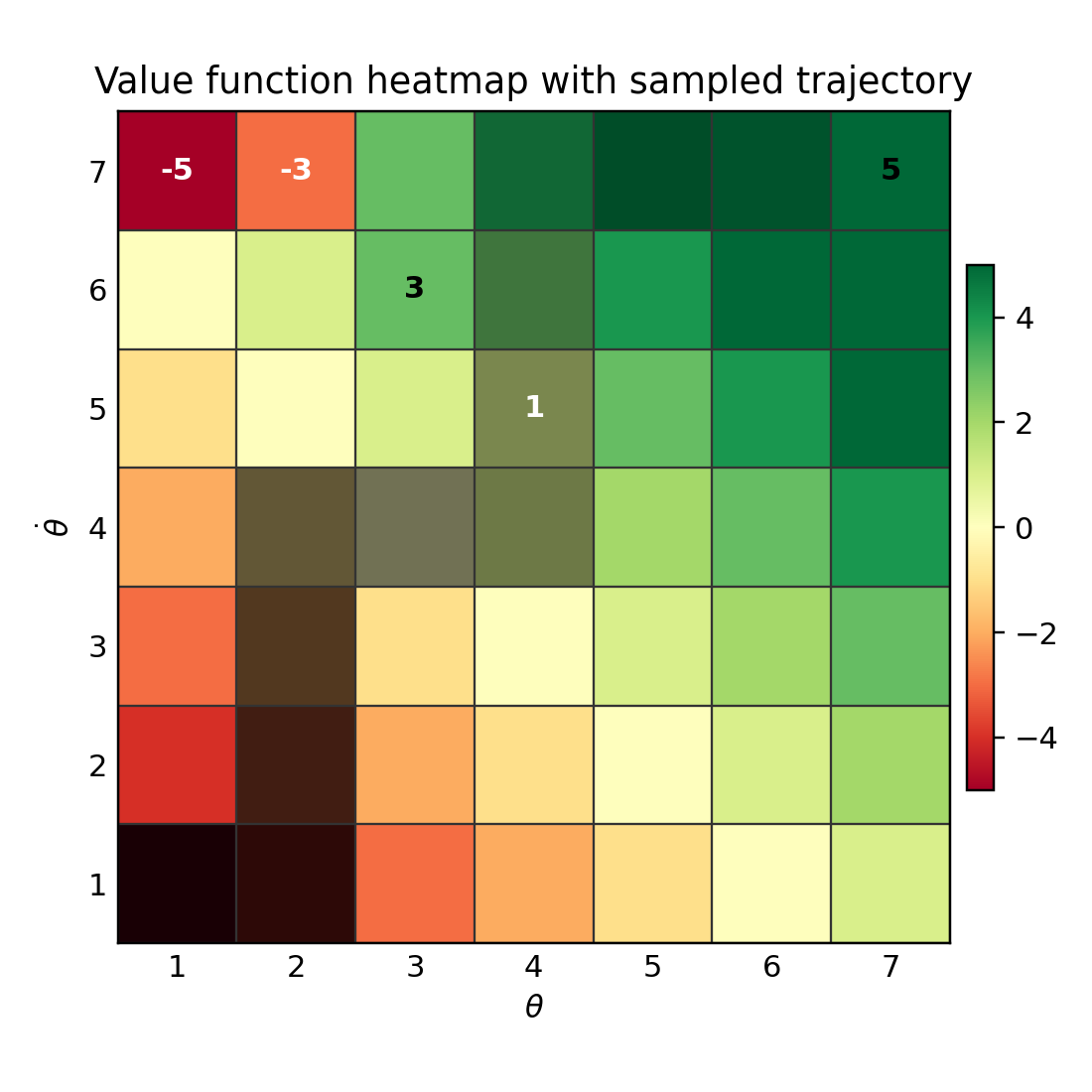
We initialize a policy \(\pi\) (often \(\varepsilon\)-soft). Run an episode: \(\pi: S_0, A_0, R_1, \dots, S_{T-1}, A_{T-1}, R_T\) Imagine a grid-world where states are angle and angular rate (these could represent anything in practice). We play an episode and obtain a trajectory (dark to pale over time).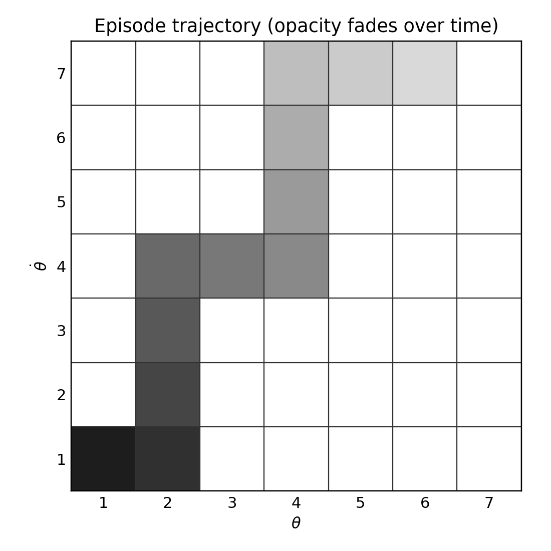 Work backward from the terminal state using returns (the return for a state-action pair is the discounted sum of rewards after taking that pair): $$ G_t(s_t, a_t) = R_{t+1} + \gamma G_{t+1}, $$ with \(G_{t+1}\) the accumulated return beyond the next step. Example along a path: $$ G_{T-1}=5+0=5,\qquad G_{T-2}=5+\gamma\cdot5,\dots $$
One observed return is not yet a value function
For an episode ending at \(T\), $$G_t=\sum_{k=t}^{T-1}\gamma^{k-t}R_{k+1},\qquad Q^\pi(s,a)=\mathbb E_\pi[G_t\mid S_t=s,A_t=a].$$ The backward pass computes the first quantity. Averaging many suitable returns estimates the second. The heatmap from a single trajectory is therefore an illustration of return propagation, not an exact map of \(Q^\pi\).
If rewards are 1, 0, and 2 with \(\gamma=0.9\), the three returns are 2.62, 1.8, and 2. A repeated state-action pair raises a bookkeeping question. First-visit MC uses only the earliest occurrence of that pair in each episode; every-visit MC uses all occurrences. When computing returns backwards, the first occurrence encountered is the last chronological visit, so simply keeping a reverse-pass seen-set would implement last-visit selection instead.
Unifying samples across episodes.
For each state-action pair, store the list of observed returns and take the average: $$ Q(S_t, A_t) = \text{Average}(G_t). $$What converges when the policy stays fixed?
For independent episodes under a fixed policy, first-visit returns for a given pair are samples of the same conditional return distribution. If its variance is \(\sigma_G^2\), the average of \(n\) such returns has variance \(\sigma_G^2/n\). Every-visit returns within an episode are correlated; they cannot all be counted as independent observations when constructing uncertainty intervals.
During control the policy changes, so old and new returns need not have the same expectation. An action followed by a poor policy can have a low return even if it becomes valuable under a better continuation policy. This is why prediction convergence for a fixed policy and convergence of an interleaved control algorithm are separate statements. More episodes alone do not remove every coverage or policy-change issue.
Memory considerations.
\(N\) episodes of length \(M\) imply \(N \times M\) stored returns. To avoid unbounded memory, use an incremental mean: $$ Q(s_t, a_t) = \frac{(N-1) \cdot Q_{\text{old}}(s_t, a_t)}{N} + \frac{G_t}{N}, $$ which only needs a running mean and a visit count per state-action pair.Fixed step size (forgetting factor).
Recent returns are often more informative than early ones. Replace \(1/N\) with a constant step size \(\alpha\): $$ Q(s_t, a_t) \leftarrow Q(s_t, a_t) + \alpha \big[G_t - Q(s_t, a_t)\big]. $$ This discounts old evidence, which can help track changing returns at the cost of persistent sampling noise.The weights hidden inside a constant step size
Index the successive returns for one pair by \(G_1,\ldots,G_n\). Repeatedly expanding the constant-step update yields $$Q_n=(1-\alpha)^nQ_0+\alpha\sum_{i=1}^n(1-\alpha)^{n-i}G_i.$$ Older evidence receives exponentially smaller weight. This can help track a changing policy, but it also means new sampling noise keeps affecting the estimate. It is not a universal reduction in training time.
For independent stationary returns with variance \(\sigma_G^2\), the long-run variance of this estimate is \(\alpha\sigma_G^2/(2-\alpha)\). A small constant step size smooths noise but adapts slowly. A sample mean instead gives every observed return equal weight and its variance tends to zero as the sample count grows. These choices answer different questions: estimating one stationary expectation versus following a moving one.
Monte Carlo policy iteration (on \(Q\)).
Combine Q-updates with policy improvement:- Policy evaluation: update \(Q\) using the returns from the episode.
- Policy improvement: \(\pi(s)\in\arg\max_a Q(s,a)\).
\(\varepsilon\)-soft policy.
$$ \pi(a \mid S_t) \leftarrow \begin{cases} 1 - \varepsilon + \varepsilon / |A(S_t)|, & a = A^* \\ \varepsilon / |A(S_t)|, & a \neq A^* \end{cases} $$ This keeps exploring while favoring the current best action. In simulation you can also use exploring starts (sample random initial state-action pairs) to improve coverage. Fixed-policy prediction and control have different convergence requirements. With fixed positive exploration, the behaviour remains epsilon-soft even after its value estimates stabilize.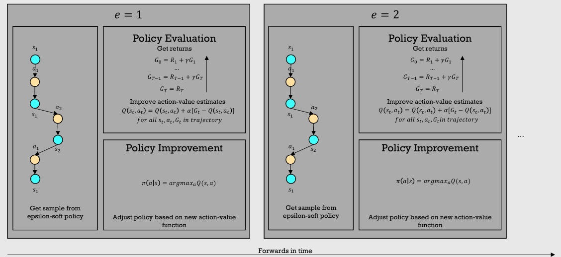
Properties and caveats.
- First technique in this series that learns directly from experience (no model required).
- Updates move backward from the episode's end, one step at a time.
- Sample inefficient: needs full episodes and only updates visited state-action pairs.
- Ambiguity can persist about which actions caused success (e.g., two pendulum trajectories ending at the same setpoint).
Coverage, policy changes, and off-policy returns
With a fixed positive \(\varepsilon\), the policy is constrained to assign every action at least \(\varepsilon/|\mathcal A(s)|\) probability. Even perfect values do not turn it into a purely greedy policy. To discuss convergence toward unconstrained optimal control, one must specify an exploration schedule and a control scheme with the required guarantees; exploration at visited states alone does not prove every relevant state is reached.
If episodes instead come from a behaviour policy \(b\), their returns generally estimate that policy rather than a different target policy \(\pi\). For a fixed state-action pair at time \(t\), future action choices can be corrected by a likelihood ratio $$\rho_{t+1:T-1}=\prod_{k=t+1}^{T-1}\frac{\pi(A_k\mid S_k)}{b(A_k\mid S_k)},\qquad Q^\pi(s,a)=\mathbb E_b[\rho_{t+1:T-1}G_t\mid s,a].$$ We start the product after \(t\) because the initial action is already conditioned on. Target-policy actions must have positive behaviour probability wherever they can occur. Long products can have enormous variance, which makes unrestricted reuse of old episodes much less straightforward than storing more data.
Blackjack is a useful episodic example because a hand genuinely ends. Win rate alone nevertheless discards the distinction between losses and draws. With rewards +1, −1, and 0, expected undiscounted return is \(\Pr(\mathrm{win})-\Pr(\mathrm{loss})\). With \(\gamma<1\), even that identity changes because the delay until the final reward matters. Evaluate the quantity that matches the objective you trained.
Worked example: Monte Carlo control on Blackjack (Gymnasium).
Below is a walk-through ofpython_scripts/rl_4_montecarlo_control.py, which learns \(Q(s,a)\) for the Blackjack-v1 environment using first-visit MC control with an \(\varepsilon\)-soft policy. 1) Imports and entry point. Main sets up the environment, agent, training loop, and win-rate tracking. import numpy as np
import gymnasium as gym
import matplotlib.pyplot as plt
if __name__ == "__main__":
    env = gym.make("Blackjack-v1")
    agent = Agent(eps=0.001)
    n_episodes = 200_000
    win_lose_draw = {-1: 0, 0: 0, 1: 0}
    win_rates = []

    for i in range(n_episodes):
        if i > 0 and i % 1000 == 0:
            win_rates.append(win_lose_draw[1] / i)
        if i % 50_000 == 0:
            print("starting episode", i, "winrate %.3f" % (win_rates[-1] if win_rates else 0.0))

        state, _ = env.reset()
        done = False
        while not done:
            action = agent.choose_action(state)
            next_state, reward, terminated, truncated, _ = env.step(action)
            if truncated and not terminated:
                raise RuntimeError("MC needs a complete hand; do not treat a cutoff as terminal")
            done = terminated or truncated
            agent.memory.append((state, action, reward))
            state = next_state

        agent.update_Q()
        win_lose_draw[reward] += 1

    plt.plot(win_rates)
plt.show()class Agent:
def __init__(self, eps=0.1, gamma=0.99):
self.Q = {}
self.sum_space = [i for i in range(4, 22)]
self.dealer_show_card_space = [i + 1 for i in range(10)]
self.ace_space = [False, True]
self.action_space = [0, 1] # stick or hit
self.state_space = []
self.returns = {}
self.pairs_visited = {}
self.memory = []
self.gamma = gamma
self.eps = eps
self.init_vals()
self.init_policy() def init_vals(self):
for total in self.sum_space:
for card in self.dealer_show_card_space:
for ace in self.ace_space:
state = (total, card, ace)
self.state_space.append(state)
for action in self.action_space:
self.Q[(state, action)] = 0.0
self.returns[(state, action)] = []
self.pairs_visited[(state, action)] = 0
def init_policy(self):
policy = {}
n = len(self.action_space)
for state in self.state_space:
policy[state] = [1 / n for _ in range(n)]
self.policy = policy def choose_action(self, state):
return np.random.choice(self.action_space, p=self.policy[state]) def update_Q(self):
for idx, (state, action, _) in enumerate(self.memory):
if self.pairs_visited[state, action] == 0:
self.pairs_visited[state, action] += 1
G = 0.0
discount = 1.0
for _, _, reward in self.memory[idx:]:
G += reward * discount
discount *= self.gamma
self.returns[state, action].append(G)
for state, action, _ in self.memory:
self.Q[state, action] = np.mean(self.returns[state, action])
self.update_policy(state)
for sa in self.pairs_visited:
self.pairs_visited[sa] = 0
self.memory = []
def update_policy(self, state):
actions = [self.Q[(state, a)] for a in self.action_space]
a_max = int(np.argmax(actions))
n_actions = len(self.action_space)
self.policy[state] = [
1 - self.eps + self.eps / n_actions if a == a_max else self.eps / n_actions
for a in self.action_space
]if __name__ == "__main__":
env = gym.make("Blackjack-v1")
agent = Agent(eps=0.001)
n_episodes = 200_000
win_lose_draw = {-1: 0, 0: 0, 1: 0}
win_rates = []
for i in range(n_episodes):
if i > 0 and i % 1000 == 0:
win_rates.append(win_lose_draw[1] / i)
if i % 50_000 == 0:
print("starting episode", i, "winrate %.3f" % (win_rates[-1] if win_rates else 0.0))
state, _ = env.reset()
done = False
while not done:
action = agent.choose_action(state)
next_state, reward, terminated, truncated, _ = env.step(action)
if truncated and not terminated:
raise RuntimeError("MC needs a complete hand; do not treat a cutoff as terminal")
done = terminated or truncated
agent.memory.append((state, action, reward))
state = next_state
agent.update_Q()
win_lose_draw[reward] += 1
plt.plot(win_rates)
plt.show()Value prediction instead of control.
The same Monte Carlo machinery can estimate a state-value function \(V^\pi(s)\) (prediction under a fixed policy) rather than a Q-function. The return from the first visit to state \(s_t\) in an episode is $$ G_t = \sum_{k=0}^{T-t-1} \gamma^k r_{t+k+1}, $$ and the first-visit MC estimate is the sample average: $$ V(s) \leftarrow \frac{1}{N(s)} \sum_{i=1}^{N(s)} G^{(i)}(s), $$ or incrementally, $$ V(s) \leftarrow V(s) + \alpha \big[G_t - V(s)\big]. $$ Below is a Blackjack example frompython_scripts/rl_4_montecarlo_prediction.py that learns \(V^\pi\) for a fixed (non-learning) policy. 1) Setup: value tables and a simple policy. We track \(V\), returns, and first-visit flags for every Blackjack state. import numpy as np
import gymnasium as gym
class Agent:
def __init__(self, gamma=0.99):
self.V = {}
self.sum_space = [i for i in range(4, 22)]
self.dealer_show_card_space = [i + 1 for i in range(10)]
self.ace_space = [False, True]
self.state_space = []
self.returns = {}
self.states_visited = {}
self.memory = []
self.gamma = gamma
self.init_vals()
def init_vals(self):
for total in self.sum_space:
for card in self.dealer_show_card_space:
for ace in self.ace_space:
state = (total, card, ace)
self.V[state] = 0.0
self.returns[state] = []
self.states_visited[state] = 0
self.state_space.append(state)
def policy(self, state):
total, _, _ = state
return 0 if total >= 20 else 1 def update_V(self):
for idx, (state, _) in enumerate(self.memory):
if self.states_visited[state] == 0:
self.states_visited[state] += 1
G = 0.0
discount = 1.0
for _, reward in self.memory[idx:]:
G += reward * discount
discount *= self.gamma
self.returns[state].append(G)
for state, _ in self.memory:
self.V[state] = np.mean(self.returns[state])
for state in self.state_space:
self.states_visited[state] = 0
self.memory = []if __name__ == "__main__":
env = gym.make("Blackjack-v1")
agent = Agent()
n_episodes = 500_000
for i in range(n_episodes):
if i % 50_000 == 0:
print("starting episode", i)
state, _ = env.reset()
done = False
while not done:
action = agent.policy(state)
next_state, reward, terminated, truncated, _ = env.step(action)
if truncated and not terminated:
raise RuntimeError("MC needs a complete hand; do not treat a cutoff as terminal")
done = terminated or truncated
agent.memory.append((state, reward))
state = next_state
agent.update_V()
print(agent.V[21, 3, True]) # near win
print(agent.V[4, 1, False]) # poor hand vs dealer ace