DDPG connects a continuous-action policy to a learned critic. Its weakness is also clear: the actor can exploit mistakes in that critic. The final course module develops TD3 and includes a SAC implementation. These methods share replay and learned value estimates, but they change the learning process in different ways.
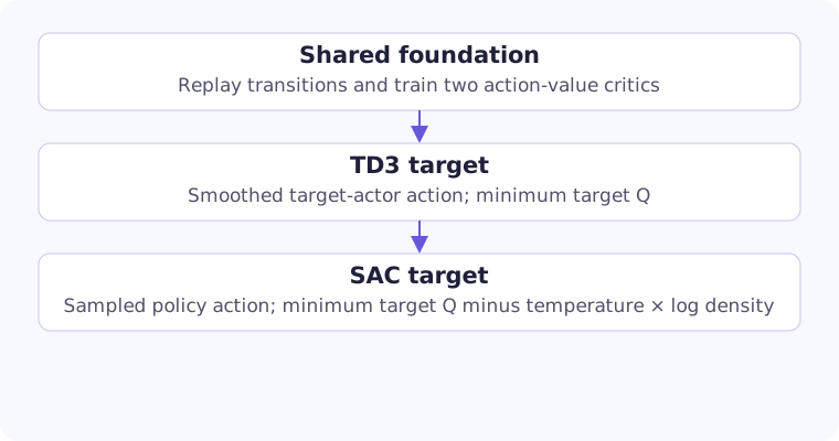
TD3 makes three targeted changes
Twin Delayed Deep Deterministic Policy Gradient, or TD3, retains a deterministic actor and introduces twin critics, delayed policy updates, and target-policy smoothing. Target networks were already part of DDPG; their existence alone is not a new TD3 contribution.
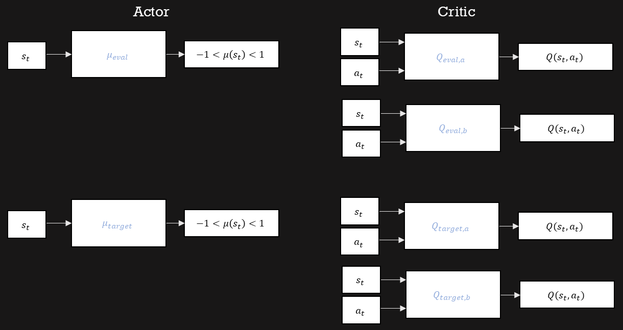
The two online critics \(Q_{\phi_1}\) and \(Q_{\phi_2}\) have separate parameters and corresponding target copies. Use the smaller target estimate in the bootstrap. The minimum discourages the actor from benefiting from a high error in just one estimate, but can introduce underestimation. Correlated critic errors can still survive.
Train the critics more frequently than the actor. At the chosen policy-update interval, update the actor and softly update all target networks. For an interval of two, actor updates occur on critic steps 2, 4, 6, and so on. This is an update counter, not necessarily an episode or epoch counter.
TD3: Fujimoto, van Hoof, and Meger
The six networks in the slide can be read as two sets of three: an actor and two critics for online learning, and corresponding target copies. The distinction matters when implementing the delayed updates: online critics learn more frequently than the actor and target copies.
Why taking a minimum changes the direction of estimation bias
At a fixed state-action pair, write two estimates as \(Q_1=q+e_1\) and \(Q_2=q+e_2\). The identity $$\min(Q_1,Q_2)=q+\frac{e_1+e_2-|e_1-e_2|}{2}$$ shows what the minimum does. If both errors have mean zero, its expected bias is \(-\tfrac12\mathbb E|e_1-e_2|\), which is nonpositive. This is a mechanism for counteracting overestimation, not a magically unbiased value estimate. If the errors are identical, the minimum cannot remove their shared error.
For independent errors that are equally likely to be +1 or −1, the minimum's mean is −0.5, mirroring the +0.5 maximum bias in the DQN example. Real critics are trained on overlapping data and common targets, so their errors are neither independent nor necessarily centered. Separate initialization can make their predictions differ, but does not justify treating them as independent uncertainty samples.
TD3's losses make its roles explicit: $$L_{Q_i}=\mathbb E_{\mathcal D}[(Q_{\phi_i}(s,a)-y)^2],\qquad L_\mu=-\mathbb E_{s\sim\mathcal D}[Q_{\phi_1}(s,\mu_\theta(s))].$$ Both critics fit the conservative target; the standard actor update follows the first online critic. Delaying actor updates gives the value estimators additional updates between policy changes. It addresses a feedback problem in optimization, not a mathematical guarantee that the critics have converged before each actor step.
Target smoothing is different from exploration
Before constructing the target, perturb the target actor’s proposed next action: $$\tilde a=\operatorname{clip}\big(\mu_{\bar\theta}(s^{\prime})+\operatorname{clip}(\epsilon,-c,c),a_{\min},a_{\max}\big),\quad\epsilon\sim\mathcal N(0,\sigma^2I).$$ Then use $$y=r+\gamma(1-d)\min_{i=1,2}Q_{\bar\phi_i}(s^{\prime},\tilde a).$$
The inner clipping limits the perturbation; the outer clipping respects the action bounds. Sampling a noise tensor with the action tensor’s shape provides a perturbation for every sample and action dimension. Adding one scalar to a whole minibatch creates a different correlation structure.
Exploration noise changes the actions sent to the environment. Target smoothing changes hypothetical actions used during learning. Its purpose is to make a narrow, erroneously high Q peak less attractive to optimize. It is not a filter on the deployed controller’s output.
import torch

def td3_target(target_actor, target_q1, target_q2,
               next_states, rewards, terminated, low, high,
               gamma=0.99, noise_std=0.2, noise_clip=0.5):
    # low and high are tensors in the same units/device as actor outputs.
    with torch.no_grad():
        action = target_actor(next_states)
        noise = (torch.randn_like(action) * noise_std).clamp(-noise_clip, noise_clip)
        action = torch.maximum(low, torch.minimum(high, action + noise))
        q = torch.minimum(target_q1(next_states, action),
                          target_q2(next_states, action)).squeeze(-1)
        return rewards + gamma * (~terminated.bool()).float() * q

# After each critic update:
# if critic_steps % policy_delay == 0:
#     update_actor()        # minimize -Q1(states, actor(states)).mean()
#     soft_update_targets()
The example noise magnitudes are illustrative and must be interpreted in the actor’s action units. Each critic minimizes its own squared error to the same detached target. The usual actor objective uses the first critic; squaring its Q-values would optimize a different objective.
Smoothing evaluates a neighborhood of actions
Ignoring clipping briefly, the noise-averaged target queries \(\mathbb E_\epsilon[Q(s',\mu(s')+\epsilon)]\). A second-order expansion with small zero-mean isotropic noise gives $$\mathbb E_\epsilon[Q(s',a+\epsilon)]\approx Q(s',a)+\frac{\sigma^2}{2}\operatorname{tr}(\nabla_a^2Q(s',a)).$$ At a sharp local maximum the curvature is negative, so nearby perturbations lower the averaged estimate. A broad plateau changes less. The actual TD3 target also uses a minimum and two clipping operations, so this expansion explains the local intuition without being an exact formula for its complete target.
Each sampled perturbation estimates that local average. Increasing its scale changes which action neighborhood is evaluated, and clipping can make noise asymmetric near action limits. Consequently, the smoothing scale must be understood in the same units as the actor's outputs. It is a training target design, not a bound on how quickly deployed motor commands can change between time steps.
SAC changes what the policy optimizes
Soft Actor-Critic, or SAC, learns a stochastic policy with an entropy-regularized objective: $$J=\mathbb E\left[\sum_t\gamma^t\big(R_{t+1}+\alpha\mathcal H(\pi(\cdot\mid S_t))\big)\right].$$ The temperature \(\alpha\) controls the reward–entropy trade-off. It is not the optimizer learning rate, even though code sometimes uses the same Greek letter for both.
SAC does not merely add random noise to a deterministic actor. It learns distribution parameters, and the entropy term affects the value targets and policy objective. Entropy encourages spread; it is not a direct measurement of model uncertainty or a guarantee that the policy will escape every poor solution.
The supplied SAC script uses a separate value network and target value network, reflecting an earlier formulation. Here we write the closely related form with twin Q-target networks and no separate value network. The target and density equations are stated explicitly so the two implementations are not accidentally mixed.
Original SAC paper: Haarnoja and colleagues
Entropy turns greedy improvement into a distribution over actions
For a fixed state and discrete actions, consider maximizing \(\sum_a\pi(a)Q(a)+\alpha H(\pi)\) subject to \(\sum_a\pi(a)=1\). Differentiating its Lagrangian gives \(Q(a)-\alpha(\log\pi(a)+1)+\lambda_0=0\). Normalization then yields $$\pi^*(a\mid s)=\frac{\exp(Q(s,a)/\alpha)}{Z(s)},\qquad Z(s)=\sum_b\exp(Q(s,b)/\alpha).$$ The best regularized value is \(\alpha\log Z(s)\). Small positive temperature favors near-maximal actions strongly; larger temperature makes differences in Q less decisive.
For example, with action values 2 and 1, temperature 1 assigns the better action probability \(e^2/(e^2+e)\approx0.731\). At temperature 0.1 its probability is about 0.99995. Reward scale therefore matters: doubling all Q-values at fixed temperature makes the policy more concentrated. Scaling rewards and temperature together preserves this local trade-off.
In continuous action spaces the normalization becomes an integral over the action domain. SAC fits a parameterized policy instead of evaluating that integral exactly. Entropy is differential entropy, \(\mathcal H(\pi)=-\int\pi(a)\log\pi(a)\,da\); unlike discrete entropy, it can be negative and depends on the units used to measure actions. This is why the density transformation in the next section matters.
The soft target and policy loss
Sample \(a^{\prime}\sim\pi_\theta(\cdot\mid s^{\prime})\). In the formulation used here, the detached Q target is $$y=r+\gamma(1-d)\left[\min_i Q_{\bar\phi_i}(s^{\prime},a^{\prime})-\alpha\log\pi_\theta(a^{\prime}\mid s^{\prime})\right].$$ The actor minimizes $$L_\pi=\mathbb E\left[\alpha\log\pi_\theta(a\mid s)-\min_iQ_{\phi_i}(s,a)\right],\quad a\sim\pi_\theta(\cdot\mid s).$$
For the actor update, sample through a differentiable reparameterization of the distribution. Hold critic parameters fixed, while retaining gradients through the action input. For the Q target, neither the sampled next action nor the target critic is differentiated. These are different uses of otherwise similar computations.
A fixed temperature gives a clear teaching example. Automatic temperature adjustment is an additional optimization problem with a chosen target entropy; it should not be implied by an implementation that only scales rewards.
Deriving the soft Bellman target and actor objective
Use the convention that soft Q includes the current reward and entropy from subsequent decisions, while soft V also includes the current decision's entropy: $$V^\pi(s)=\mathbb E_{a\sim\pi}[Q^\pi(s,a)-\alpha\log\pi(a\mid s)],\qquad Q^\pi(s,a)=\mathbb E[r+\gamma(1-d)V^\pi(s')\mid s,a].$$ Substituting the first equation into the second gives the sampled soft target above. Placing the entropy term inconsistently at both the current Q reward and the next V would double count part of the objective.
At a fixed state, define the Boltzmann density \(p_Q(a)\propto\exp(Q(s,a)/\alpha)\), assuming its normalization is finite. Then $$\alpha D_{\mathrm{KL}}(\pi_\theta\|p_Q)=\mathbb E_{a\sim\pi_\theta}[\alpha\log\pi_\theta(a\mid s)-Q(s,a)]+\alpha\log Z(s).$$ Holding the critic fixed makes the last term constant with respect to the actor. Minimizing the policy loss thus fits the policy toward a distribution that favors high values while retaining the entropy trade-off. Twin-critic minima provide the practical Q estimate, rather than changing the logic of this regularized improvement step.
To differentiate the sampled actor objective, write \(a=f_\theta(s,\epsilon)\) with parameter-independent noise \(\epsilon\). Backpropagation then differentiates both the log density and the critic evaluated at that action. This pathwise derivative differs from REINFORCE's score-function estimator: the critic now supplies a differentiable surrogate for how changing the action changes expected return. The environment itself still need not be differentiable.
A bounded action needs a corrected log density
A Gaussian policy is unbounded. To obtain bounded actions, sample \(u=\mu+\sigma\odot\epsilon\), let \(z=\tanh(u)\), and map \(a=m+c\odot z\), where \(m\) is the action midpoint and \(c\) its positive half-range. The probability density must account for both transformations: $$\log\pi(a\mid s)=\sum_j\left[\log\mathcal N(u_j;\mu_j,\sigma_j)-\log(1-\tanh^2(u_j))-\log c_j\right].$$
The tanh correction uses the normalized tanh output, not the final scaled action. For a pendulum with actions outside −1 to 1, placing the scaled action inside log(1 − action²) can produce invalid values. The affine scaling term also matters when reporting densities in environment action units.
import math
import torch
from torch.distributions import Normal
from torch.nn import functional as F

def squashed_sample(mean, log_std, low, high):
    # All tensors share a device; high > low in every action dimension.
    scale, midpoint = (high - low) / 2, (high + low) / 2
    normal = Normal(mean, log_std.clamp(-20, 2).exp())
    u = normal.rsample()  # keep a gradient path into mean and standard deviation
    action = midpoint + scale * torch.tanh(u)
    # Stable log(1 - tanh(u)**2), including near saturation:
    log_jacobian = 2 * (math.log(2) - u - F.softplus(-2*u))
    log_probability = (normal.log_prob(u) - log_jacobian - scale.log()).sum(-1)
    return action, log_probability
The function is a distribution-sampling kernel, not a complete SAC agent. It uses finite bounds and one independent Gaussian dimension per action component before squashing. Return a single summed log density per sample so it aligns with scalar critic values.
Change of variables explains the density correction
For a one-to-one differentiable transformation \(a=f(u)\), conservation of probability gives \(\pi(a)\,da=p_U(u)\,du\), hence $$\log\pi(a)=\log p_U(u)-\log\left|\det\frac{\partial a}{\partial u}\right|.$$ For componentwise tanh and affine scaling, the Jacobian is diagonal with entries \(c_j(1-\tanh^2u_j)\). Taking its log determinant yields the sum of corrections in the equation above. Tanh maps finite latent samples into the open action interval; saturation makes the Jacobian small, not negative.
The base diagonal-Gaussian log density is $$\log p_U(u)=-\frac12\sum_j\left[\left(\frac{u_j-\mu_j}{\sigma_j}\right)^2+2\log\sigma_j+\log(2\pi)\right].$$ The implementation sums over action components to obtain one log density per sample. Summing over the minibatch instead would mix independent training examples and break alignment with the scalar Q predictions.
As a scalar check, a standard normal sampled at \(u=0\) has log density about −0.91894. With action half-range \(c=2\), the tanh derivative at zero is 1 and the transformed log density is \(-0.91894-\log2\approx-1.61209\). Doubling the action units spreads the density over twice the interval. This shift is expected and explains why entropy targets must use the same action convention as the reported log densities.
Automatic temperature tuning can be motivated by a minimum expected entropy constraint \(\mathbb E[-\log\pi(a\mid s)]\ge\mathcal H_{\mathrm{target}}\). With the sampled log density detached, a dual temperature loss is $$L_\alpha=\mathbb E[-\alpha(\log\pi(a\mid s)+\mathcal H_{\mathrm{target}})].$$ Parameterizing \(\alpha=\exp\xi\) keeps it positive. If current entropy is below the target, gradient descent on this loss increases temperature; above target, it decreases it. The desired entropy is a chosen constraint, not an automatically inferred measure of useful exploration. The displayed sampling kernel does not include this additional optimizer.
SAC with temperature adjustment: Haarnoja and colleagues
Compare mechanisms before comparing scores
| Method | Policy | Key change |
|---|---|---|
| DDPG | Deterministic; external training noise | Actor optimized through a replay-trained critic |
| TD3 | Deterministic; external training noise | Twin targets, delayed actor updates, target smoothing |
| SAC | Learned stochastic distribution | Entropy enters policy and critic objectives |
The course uses different environments to demonstrate DDPG, TD3, and SAC. Scores from continuous LunarLander, a walker, and Pendulum are not a controlled algorithm comparison. To compare algorithms, use the same task, action scaling, interaction budget, evaluation protocol, and several random seeds.
Record return variability, environment steps, gradient updates, and computation time. For SAC, state whether evaluation samples actions or uses the squashed mean. For TD3, record both policy-delay and target-update settings. Training loss alone remains insufficient for all three methods.
This completes the progression in the prepared course material: tables, function approximation, learned action values, direct policy gradients, and critics that guide continuous actions. The common discipline is to identify the prediction, its target, and the exact gradient path before interpreting a learning curve.
Adapted from my reinforcement learning course: module 08, slides 17–22, TD3_walker.py, and SAC_pendulum.py. The worked examples in this post are teaching examples, not benchmark results.