Use LibEMG’s offline data and filtering tools with WFDB ECG recordings, then build and evaluate an educational QRS and R-peak timing pipeline.
Download the complete runnable series (Python scripts, shared helpers and setup instructions).
Use 64-bit Python 3.11 and LibEMG 2.0.3. Keep the downloaded files together: the walkthrough uses common.py from that bundle. The figures below were generated by these scripts; results describe the stated recordings and split.
Reuse the tooling while changing the task
An ECG is a cardiac electrical recording, so gesture labels and EMG feature choices are no longer the objective. We want event times. This exercise uses external MIT-BIH Arrhythmia Database records 100 and 101, version 1.0.0, rather than claiming ECG is bundled in LibEMG’s EMG dataset catalogue. LibEMG loads the WFDB signal and supplies filtering; NumPy, SciPy and WFDB implement the detector and evaluation.
python prepare_data.py ecgRead the sampling rate, lead and units from the header. Both excerpts use the first lead, MLII, at 360 Hz in millivolts. Beat annotations include event categories; rhythm-change symbols such as “+” are not beats. The loader retains recognized beat symbols and reads only the first sixty seconds for this exercise.
import json
import numpy as np
import matplotlib.pyplot as plt
from scipy.signal import find_peaks
import wfdb
from wfdb.processing import compare_annotations
from libemg.data_handler import OfflineDataHandler, RegexFilter
from libemg.filtering import Filter
from common import DATA, OUT, savefig

BEATS = set(['N', 'L', 'R', 'B', 'A', 'a', 'J', 'S', 'V', 'r',
             'F', 'e', 'j', 'n', 'E', '/', 'f', 'Q'])
def load_record(name, seconds=60):
    path = DATA/'ecg'/name
    header = wfdb.rdheader(str(path))
    handler = OfflineDataHandler()
    handler.get_data((DATA/'ecg').as_posix(),
        [RegexFilter('/', '.hea', [name], 'record')],
        mrdf_key='p_signal', data_column=[0])
    signal = handler.data[0][:round(seconds*header.fs), 0]
    annotation = wfdb.rdann(str(path), 'atr', sampto=len(signal))
    reference = np.array([sample for sample, symbol in zip(annotation.sample, annotation.symbol)
                          if symbol in BEATS])
    return signal, float(header.fs), reference, header.sig_name[0], header.units[0]
Turn a fast QRS transition into a candidate event
The QRS complex contains a rapid voltage transition. Apply a 5–20 Hz bandpass, take a sample-wise derivative \(d[n]\), square it, and average over 120 ms: \(E[n]=W^{-1}\sum_{j=0}^{W-1}d[n-j]^2\). Squaring makes either polarity contribute positive energy; averaging groups nearby slopes into a broader event. Our implementation uses a centered convolution, so it is offline rather than causal.
Set a robust threshold from seconds 1–10: \(\theta=\mathrm{median}(E)+5\,\mathrm{median}(|E-\mathrm{median}(E)|)\). This fixed rule uses no beat labels, but it is calibrated separately to each record’s amplitude. Candidate peaks must be separated by at least 250 ms. Refine each within ±100 ms to the largest absolute filtered deflection. That produces a useful fiducial timing estimate without assuming every QRS has a positive R peak.
def detect(signal, fs):
    bp = Filter(fs)
    bp.install_filters({'name': 'bandpass', 'cutoff': [5, 20], 'order': 3})
    filtered = bp.filter(signal[:, None])[:, 0]
    derivative = np.gradient(filtered)
    width = round(.12*fs)
    energy = np.convolve(derivative**2, np.ones(width)/width, mode='same')
    # Fixed rule, calibrated without beat labels on the first ten seconds.
    calibration = energy[round(1*fs):round(10*fs)]
    median = np.median(calibration)
    mad = np.median(np.abs(calibration-median))
    threshold = median + 5*mad
    candidates, _ = find_peaks(energy, height=threshold, distance=round(.25*fs))
    radius = round(.10*fs)
    aligned = []
    for candidate in candidates:
        left, right = max(0, candidate-radius), min(len(signal), candidate+radius+1)
        aligned.append(left + np.argmax(np.abs(filtered[left:right])))
    return np.unique(aligned), filtered, energy, threshold
These constants define a simple educational detector. The 250 ms spacing can suppress closely spaced events; motion, large T waves, changing morphology or a poor calibration interval can produce false detections. Forward–backward filtering also uses future samples. Reproducing a live detector would require causal filtering, stateful thresholds and an explicit delay budget.
Compare event times one-to-one
A detection is a true positive when it can be matched to a reference beat within the timing tolerance, without reusing either event. Sensitivity is \(\mathrm{Se}=\mathrm{TP}/(\mathrm{TP}+\mathrm{FN})\); positive predictivity is \(\mathrm{PPV}=\mathrm{TP}/(\mathrm{TP}+\mathrm{FP})\). High sensitivity alone can be obtained by predicting too many peaks, so both measures matter.
results, traces = {}, {}
for name in ['100', '101']:
    signal, fs, reference, lead, units = load_record(name)
    peaks, filtered, energy, threshold = detect(signal, fs)
    # Exclude the initialization interval and a final second of filter boundary.
    lo, hi = round(10*fs), len(signal)-round(fs)
    ref = reference[(reference >= lo) & (reference < hi)]
    pred = peaks[(peaks >= lo) & (peaks < hi)]
    comparison = compare_annotations(ref, pred, window_width=round(.15*fs))
    results[name] = {'sampling_hz': fs, 'lead': lead, 'units': units,
        'evaluated_seconds': [lo/fs, hi/fs], 'tolerance_ms': 150,
        'true_positive': int(comparison.tp), 'false_positive': int(comparison.fp),
        'false_negative': int(comparison.fn),
        'sensitivity': float(comparison.sensitivity),
        'positive_predictivity': float(comparison.positive_predictivity)}
    traces[name] = (signal, fs, reference, peaks, energy, threshold)
(OUT/'08-results.json').write_text(json.dumps(results, indent=2))
print(results)
We score seconds 10–59, excluding the calibration interval and the final filter boundary. The tolerance is 150 ms. WFDB performs one-to-one annotation matching; the annotations are beat fiducials and need not coincide exactly with the chosen extremum. A 150 ms hit therefore does not establish millisecond-level R-peak accuracy.
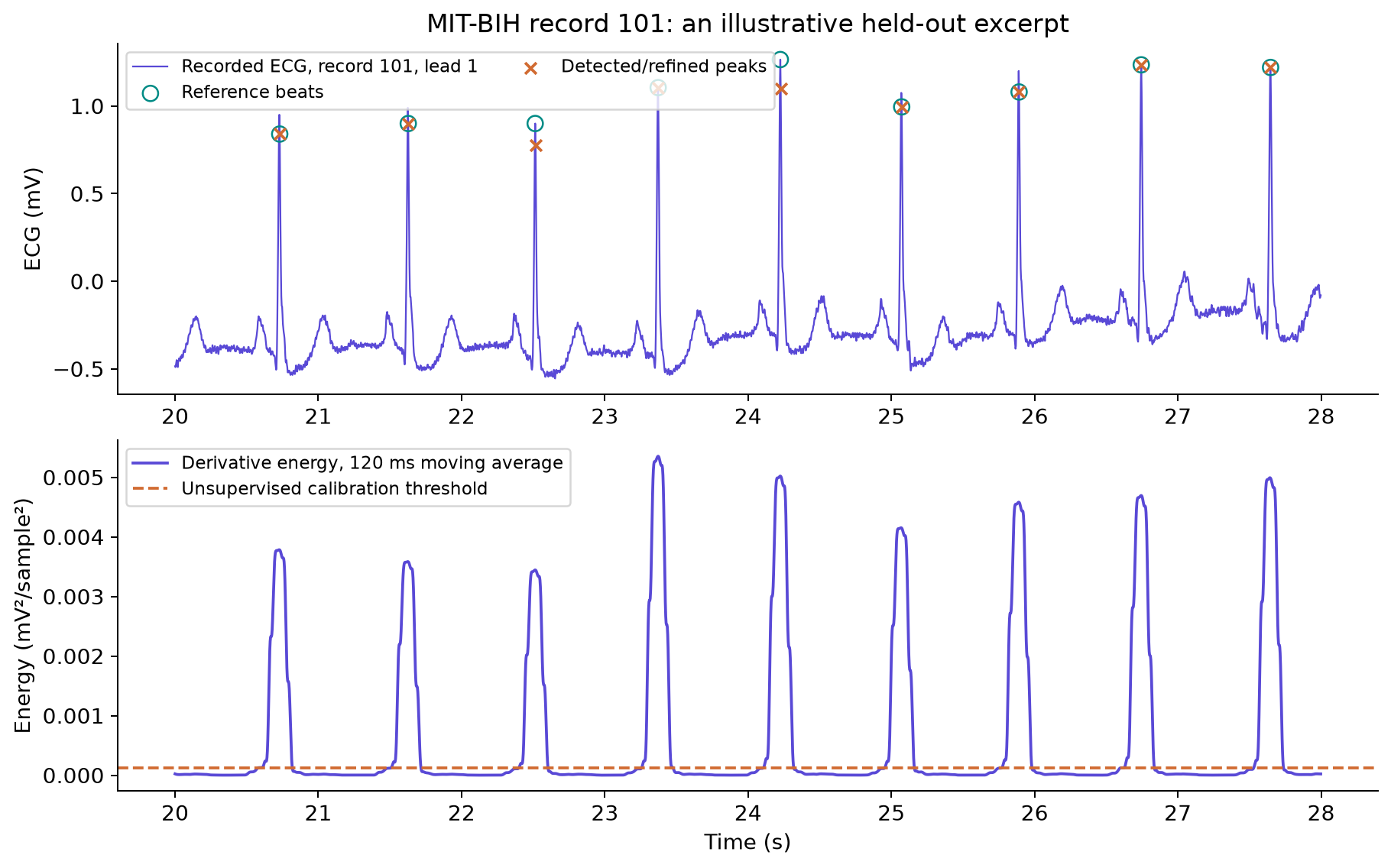
Record 100 produced 60 true positives, zero false positives and zero false negatives; record 101 produced 59, zero and zero. Sensitivity and positive predictivity were both 100% on these short evaluated intervals. That is a reproducible result on 98 seconds in total, not validation across the database, arrhythmias or clinical use.
Derive intervals without hiding detection errors
For consecutive detected sample indices \(r_i\), the interval is \(RR_i=(r_{i+1}-r_i)/f_s\) seconds and instantaneous rate is \(60/RR_i\) beats per minute. A missed beat can roughly double an interval; an extra detection can split one into two. Inspect detections before interpreting interval statistics. Detecting beat times is separate from classifying beat morphology or diagnosing rhythm.
signal, fs, reference, peaks, energy, threshold = traces['101']
rr_seconds = np.diff(peaks)/fs
instantaneous_bpm = 60/rr_seconds
# Intervals inherit missed/extra detections; do not interpret these as diagnoses.
Attribute the recording and extend the evaluation
ECG data: Moody and Mark, MIT-BIH Arrhythmia Database, version 1.0.0, PhysioNet, DOI 10.13026/C2F305, under the Open Data Commons Attribution License v1.0. PhysioNet is described by Goldberger et al. (2000), Circulation 101(23), e215–e220. The companion downloader uses the official PhysioNet public mirror and records source URLs and checksums.
Try it yourself
Evaluate longer intervals without retuning on their annotations. Report false positives and false negatives by record, then tighten the timing tolerance and plot matched timing errors. Choose a difficult example and explain which detector assumption failed instead of changing several parameters at once.
Run the full companion script to regenerate the figures and machine-readable results:
python 08_ecg.pyLibEMG documentation: offline data and metadata
LibEMG documentation: filtering