Derive two model-based estimators and test their assumptions: Wiener filtering for a noisy waveform and Kalman filtering for a changing amplitude state.
Download the complete runnable series (Python scripts, shared helpers and setup instructions).
Use 64-bit Python 3.11 and LibEMG 2.0.3. Keep the downloaded files together: the walkthrough uses common.py from that bundle. The figures below were generated by these scripts; results describe the stated recordings and split.
Decide what the hidden quantity is
A denoising method needs a target. Estimating a signed EMG waveform and tracking its slowly changing amplitude are different problems. This lesson uses synthetic signals with known references so that estimation error can be measured. It does not present synthetic improvement as a result on recorded EMG. NumPy and SciPy implement these estimators; LibEMG 2.0.3 does not provide dedicated Wiener or Kalman filters.
Derive a frequency-dependent Wiener gain
Let \(Y=S+V\), where signal and additive noise are zero-mean, stationary and uncorrelated. For a frequency-dependent linear estimate \(\widehat S=GY\), the expected squared error is \(|G-1|^2P_s+|G|^2P_v\). Minimizing with respect to the gain gives \(G(f)=P_s(f)/(P_s(f)+P_v(f))\). Signal-dominated frequencies are retained; noise-dominated frequencies are attenuated.
We estimate observed and noise spectra from an independent calibration simulation, subtract them with a nonnegative floor, and interpolate the gain onto the test FFT bins. The test reference and noise are newly drawn. Knowing the simulated calibration noise makes the assumptions explicit; in a recording, a rest segment is not automatically an observation of pure measurement noise.
import json
import numpy as np
import matplotlib.pyplot as plt
from scipy.signal import butter, sosfiltfilt, welch
from common import OUT, savefig

rng = np.random.default_rng(7)
fs, n = 1000, 12000
sos = butter(4, [70, 280], btype='bandpass', fs=fs, output='sos')
cal_signal = sosfiltfilt(sos, rng.normal(size=n))
cal_noise = rng.normal(scale=.8, size=n)
cal_observed = cal_signal + cal_noise
f, p_observed = welch(cal_observed, fs, nperseg=1024)
_, p_noise = welch(cal_noise, fs, nperseg=1024)
p_signal = np.maximum(p_observed - p_noise, 0)
gain = p_signal / np.maximum(p_signal + p_noise, 1e-12)

reference = sosfiltfilt(sos, rng.normal(size=n))
observed = reference + rng.normal(scale=.8, size=n)
fft_frequency = np.fft.rfftfreq(n, 1/fs)
gain_bins = np.interp(fft_frequency, f, gain)
estimate = np.fft.irfft(gain_bins * np.fft.rfft(observed), n=n)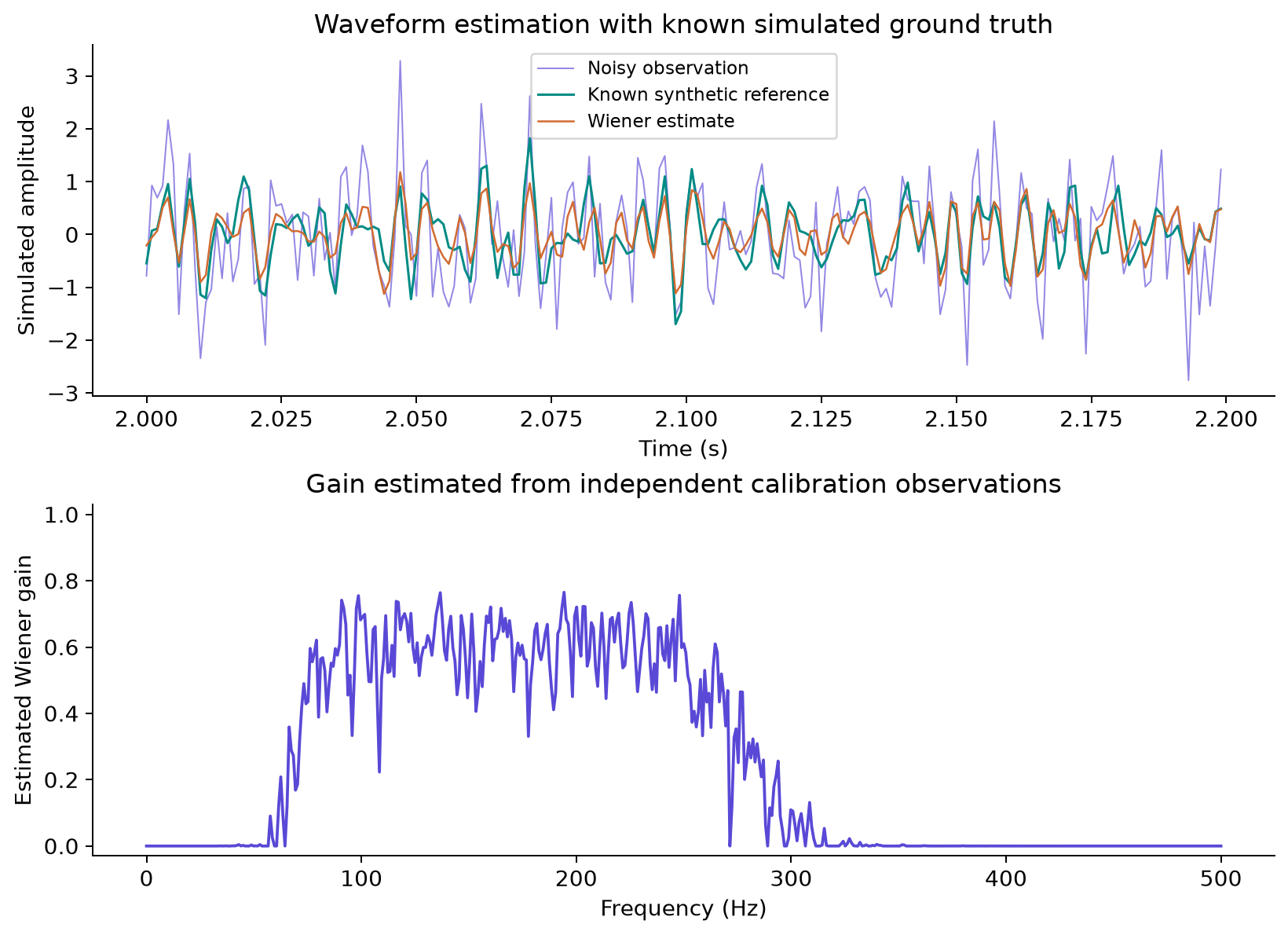
Interior mean squared error fell from 0.6365 for the noisy observation to 0.1671 for the Wiener estimate. Whole-record FFT multiplication is an offline operation with circular boundary effects; the calculation excludes one second at each end. A gain estimated from a different noise spectrum can perform much worse. Nonstationary bursts also violate the global stationary model.
SciPy’s function named signal.wiener is a local mean/variance estimator, not this explicitly constructed spectral gain. Passing a samples-by-channels matrix to a multidimensional neighbourhood method can also mix channels. Inspect the implementation and its axis assumptions before substituting a similarly named function.
Describe amplitude as a dynamical state
For an amplitude state, use \(a_t=a_{t-1}+w_t\) and measurement \(z_t=a_t+v_t\), with process variance \(Q\) and measurement variance \(R\). The prediction is \(\widehat a_t^-=\widehat a_{t-1}\), \(P_t^-=P_{t-1}+Q\). The update is \(K_t=P_t^-/(P_t^-+R)\), \(\widehat a_t=\widehat a_t^-+K_t(z_t-\widehat a_t^-)\), and \(P_t=(1-K_t)P_t^-\).
The innovation is the difference between the observed and predicted amplitude. A large gain trusts that new observation; a small gain trusts the state model. Increasing Q allows faster changes, while increasing R expresses greater uncertainty in the measurements. Their numerical values depend on amplitude units and update rate.
def kalman_envelope(measurements, process_variance, measurement_variance):
    state, variance = float(measurements[0]), measurement_variance
    estimates, gains = [], []
    for measurement in measurements:
        predicted_variance = variance + process_variance
        gain = predicted_variance / (predicted_variance + measurement_variance)
        state = state + gain * (measurement - state)
        variance = (1 - gain) * predicted_variance
        estimates.append(state)
        gains.append(gain)
    return np.array(estimates), np.array(gains)

# Controlled amplitude observations at 20 updates/s, not raw EMG samples.
time = np.arange(240)/20
amplitude = np.where(time < 4, .4, np.where(time < 8, 1.0, .55))
measurements = amplitude + rng.normal(scale=.12, size=len(time))
slow, _ = kalman_envelope(measurements, 1e-4, .12**2)
fast, _ = kalman_envelope(measurements, 1e-2, .12**2)
Measure the smoothness–response trade-off
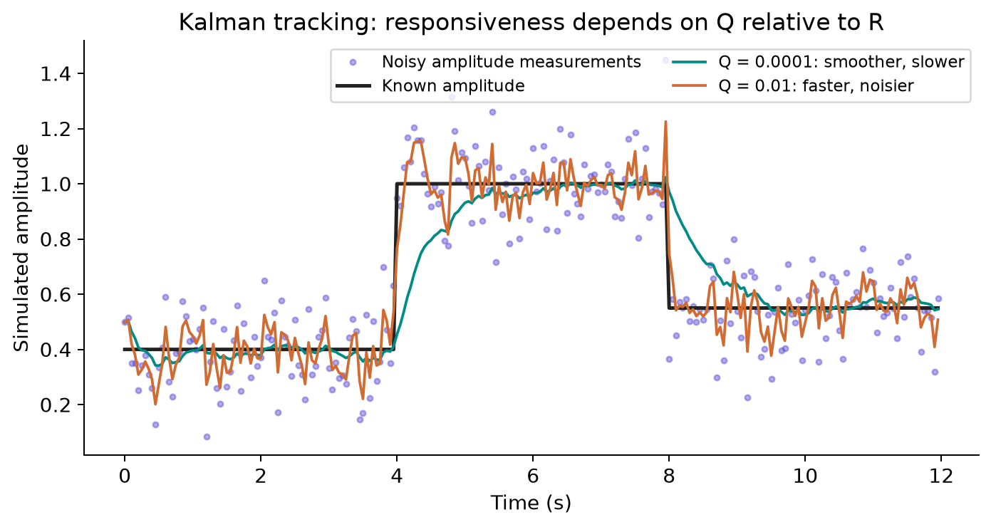
The noisy amplitude MSE was 0.01579. It became 0.01221 with Q=0.0001 and 0.00597 with Q=0.01, holding R=0.12² fixed. The faster setting is better for these particular steps, not universally. Long quiet plateaus and gradual ramps would weight the trade-off differently. The random-walk model itself does not enforce nonnegative amplitude.
Connect the state model to LibEMG features
For real data, replace synthetic measurements with one channel’s sequence of MAV or RMS values. Reset state between separate trials. Fit or justify Q and R on development recordings, and measure onset delay as well as variance. Overlapping windows produce correlated measurement errors, so the simple independent-noise Kalman model is an approximation.
from libemg.feature_extractor import FeatureExtractor
# trial_windows: (windows, channels, samples), in time order within one trial
rms = FeatureExtractor().extract_features(["RMS"], trial_windows)["RMS"]
# Q and R must be calibrated in the squared units of this RMS sequence.
tracked, gains = kalman_envelope(rms[:, 0], process_variance=Q,
                                measurement_variance=R)
That final block is an integration template: supply trial_windows and calibrated Q and R. The runnable companion provides the complete controlled experiment. Feeding the rapidly alternating raw waveform into a slow amplitude random walk would change the estimation target and usually suppress the very activity being measured.
Try it yourself
Keep the test signal fixed and change only the calibration noise spectrum for the Wiener gain. Then replace the Kalman step with a ramp. Report error and transition delay separately, and explain each change using the estimator assumptions.
Run the full companion script to regenerate the figures and machine-readable results:
python 03_advanced.pyLibEMG documentation: filtering