Use grouped forward selection and an explicit accuracy tolerance to choose a small feature subset before evaluating it on held-out recordings.
Download the complete runnable series (Python scripts, shared helpers and setup instructions).
Use 64-bit Python 3.11 and LibEMG 2.0.3. Keep the downloaded files together: the walkthrough uses common.py from that bundle. The figures below were generated by these scripts; results describe the stated recordings and split.
Define what “small” means
A compact recognizer should spend its dimensions and computation on information that helps the task. We select entire feature families across eight channels, keeping the LDA classifier fixed. One family is not always one equal-cost choice: MAV contributes eight columns, whereas order-four AR contributes 32. Deployment cost also includes feature extraction, memory and sensor count.
Remove IAV first because it is exactly 50 times MAV for these windows. This is a mathematical redundancy, not a discovery made by looking at the held-out test labels. The remaining nine families are candidates for a grouped search on the first four recording sets.
import json
import numpy as np
import matplotlib.pyplot as plt
from libemg.feature_selector import FeatureSelector
from sklearn.metrics import balanced_accuracy_score
from common import load_myo, extract, stack, held_set_scores, lda, OUT, savefig

_, _, splits = load_myo()
w, meta = splits['train']
features = extract(w)
y, groups = meta['classes'].astype(int), meta['sets'].astype(int)
# IAV is exactly N*MAV for fixed-length windows: remove it before searching.
candidates = ['MAV', 'RMS', 'VAR', 'WL', 'ZC', 'SSC', 'DASDV', 'MNF', 'AR']
Build a greedy path using held-recording folds
For selected families \(S\), evaluate \(J(S)=G^{-1}\sum_g\mathrm{Accuracy}(h_{S,-g},D_g)\), where the entire pipeline is fitted without recording group \(g\). Forward selection adds \(f^*=\arg\max_{f\notin S}J(S\cup\{f\})\). Fitting the scaler once on all groups would leak validation information into every fold; our helper fits it anew.
selected, remaining, path = [], candidates.copy(), []
while remaining:
    evaluated = []
    for candidate in remaining:
        names = selected + [candidate]
        fold_scores = held_set_scores(stack(features, names), y, groups)
        evaluated.append((float(fold_scores.mean()), candidate, fold_scores))
    # Stable candidate order breaks exact ties; do not use test outcomes.
    best = max(evaluated, key=lambda item: item[0])
    selected.append(best[1])
    remaining.remove(best[1])
    path.append({'features': selected.copy(), 'mean': best[0],
                 'fold_scores': best[2].tolist(),
                 'dimensions': stack(features, selected).shape[1]})
Greedy selection is tractable but does not guarantee the best subset: a pair that is only useful together can be missed when neither member looks good alone. Exact ties are broken by the declared candidate order. The search scores are development estimates and become optimistic as more candidates are compared.
Choose a stopping rule before inspecting test performance
Our predeclared tolerance is \(\epsilon=0.005\), or 0.5 percentage points. Choose the smallest prefix \(S_k\) satisfying \(J(S_k)\geq\max_j J(S_j)-\epsilon\). This is an accuracy-tolerance rule, not the one-standard-error rule and not an uncertainty interval. The appropriate tolerance depends on the application’s cost of errors and computation.
# Predeclared tolerance: smallest prefix within 0.5 percentage points of best CV.
tolerance = .005
best_score = max(step['mean'] for step in path)
chosen = next(step for step in path if step['mean'] >= best_score-tolerance)
chosen_names = chosen['features']
model = lda().fit(stack(features, chosen_names), y)
test_w, test_meta = splits['test']
test_features = extract(test_w, chosen_names)
prediction = model.predict(stack(test_features, chosen_names))
result = {'path': path, 'tolerance': tolerance, 'chosen': chosen_names,
          'chosen_dimensions': chosen['dimensions'],
          'test_balanced_accuracy': float(balanced_accuracy_score(test_meta['classes'], prediction))}
(OUT/'05-results.json').write_text(json.dumps(result, indent=2))
print(result)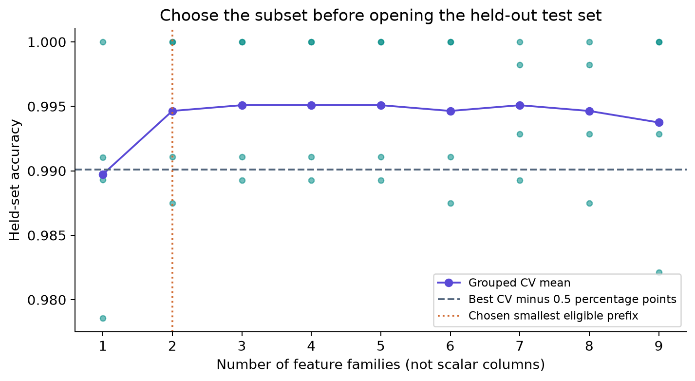
MAV alone averaged 98.97%; MAV + MNF averaged 99.46%. Adding AR increased the mean to about 99.51% while increasing dimensionality from 16 to 48. The tolerance rule selects MAV + MNF, sixteen columns. Its test balanced accuracy was 99.64%. This is a compact solution for the stated protocol, not proof that the same pair is optimal for other people or devices.
Use LibEMG’s built-in selector with its own assumptions
# LibEMG's built-in alternative uses its own default LDA, rather than our
# scaled/shrinkage pipeline. This API demonstration is not the above search.
library_scores, library_order = FeatureSelector().run_selection(
    {name: features[name].copy() for name in candidates},
    metric='accuracy', class_var=y,
    crossvalidation_var={'var': groups}, early_stop=3)
print('Built-in selector first families:', library_order)
LibEMG also provides FeatureSelector.run_selection with class labels and crossvalidation_var. That call uses its own default LDA implementation, rather than our standardized shrinkage pipeline, so its ordering need not match our custom search. In this run its first three families were MAV, MNF and RMS. Treat this as a second reproducible API example, not as the source of the preceding curve.
Keep model selection inside the evaluation boundary
The final test is evaluated once within this script, after choosing the subset. However, the teaching series deliberately reuses the Myo split across several lessons. Reading those results and repeatedly changing the method would turn that test set into development data. For a research comparison, reserve new recordings or use nested grouped cross-validation: repeat the entire feature search inside each outer training fold, then score only its outer holdout.
A feature that separates gestures because of a session-specific offset may fail after electrodes are replaced. Choose grouping to match the deployment question: held repetitions assess one kind of variation, held sessions another, and held participants another. A tiny accuracy difference is less useful than understanding which source of variation the evaluation contains.
Try it yourself
Repeat the search using a fixed scalar-column budget of sixteen rather than a family-count tolerance. Then repeat with an outer held-set loop that includes the entire selection procedure. Compare selected subsets as well as scores; unstable selections reveal interchangeable information or limited data.
Run the full companion script to regenerate the figures and machine-readable results:
python 05_selection.pyLibEMG documentation: feature selection