Train a small feature MLP and a temporal convolutional network with the same recording split, then compare learning curves and what each model is asked to learn.
Download the complete runnable series (Python scripts, shared helpers and setup instructions).
Use 64-bit Python 3.11 and LibEMG 2.0.3. Keep the downloaded files together: the walkthrough uses common.py from that bundle. The figures below were generated by these scripts; results describe the stated recordings and split.
Two representations of the same observation
The first model receives the 32 HTD features from each Myo window. The second receives eight channels by fifty time samples. “Raw” here means the stored device signal without additional feature extraction; it still includes the acquisition hardware’s bandwidth and quantization. Both models predict the same five classes from the same training, validation and test recordings.
python -m pip install torch==2.8.0 --index-url https://download.pytorch.org/whl/cpuFor each feature coordinate, standardize using \(z=(x-\mu_{\mathrm{train}})/\sigma_{\mathrm{train}}\). For raw windows, estimate one mean and standard deviation per channel across training windows and time. Do not normalize each window to unit amplitude unless intentionally discarding amplitude information; amplitude is useful for many EMG decisions.
import copy
import json
import random
import numpy as np
import matplotlib.pyplot as plt
import torch
from torch import nn
from torch.utils.data import DataLoader, TensorDataset
from sklearn.preprocessing import StandardScaler
from sklearn.metrics import balanced_accuracy_score
from common import load_myo, extract, stack, OUT, savefig

torch.set_num_threads(2)
_, _, splits = load_myo()
feature_names = ['MAV', 'ZC', 'SSC', 'WL']
feature_arrays = {name: stack(extract(w, feature_names), feature_names)
                  for name, (w, _) in splits.items()}
scaler = StandardScaler().fit(feature_arrays['train'])
feature_arrays = {name: scaler.transform(x).astype('float32')
                  for name, x in feature_arrays.items()}
train_raw = splits['train'][0]
raw_mean = train_raw.mean(axis=(0, 2), keepdims=True)
raw_std = np.maximum(train_raw.std(axis=(0, 2), keepdims=True), 1e-6)
raw_arrays = {name: ((w-raw_mean)/raw_std).astype('float32')
              for name, (w, _) in splits.items()}
labels = {name: metadata['classes'].astype('int64')
          for name, (_, metadata) in splits.items()}
Write down what the networks compute
The feature network computes \(h=\mathrm{ReLU}(W_1z+b_1)\) and logits \(\ell=W_2h+b_2\), with 32 inputs, 64 hidden units and five outputs. Its 2,437 parameters learn nonlinear combinations of descriptors whose meaning we already understand.
A temporal convolution computes \(h_{o,t}=\mathrm{ReLU}(b_o+\sum_c\sum_j w_{o,c,j}x_{c,t+j})\), with shared weights at each time position and padding at the boundaries. Two layers learn 16 then 32 temporal feature maps. Global average pooling computes \(\bar h_o=T^{-1}\sum_t h_{o,t}\); a linear layer converts those averages into five logits. The CNN has 3,669 parameters.
def make_model(kind):
    if kind == 'features':
        return nn.Sequential(nn.Linear(32, 64), nn.ReLU(), nn.Linear(64, 5))
    return nn.Sequential(
        nn.Conv1d(8, 16, kernel_size=7, padding=3), nn.ReLU(),
        nn.Conv1d(16, 32, kernel_size=5, padding=2), nn.ReLU(),
        nn.AdaptiveAvgPool1d(1), nn.Flatten(), nn.Linear(32, 5))
Temporal weight sharing makes the CNN sensitive to local patterns wherever they occur. Global averaging reduces dependence on exact timing, but it also discards some temporal ordering. A static gesture window makes this a reasonable starting point; a sequence of discrete movements could require a different representation.
Optimize cross-entropy and save the validation checkpoint
For label \(y\) and logits \(\ell\), cross-entropy is \(\mathcal L=-\ell_y+\log\sum_k e^{\ell_k}\). PyTorch CrossEntropyLoss expects logits and integer class IDs; applying softmax first would change the computation it expects. Backpropagation computes parameter gradients, and Adam updates the weights using running gradient moments.
Use batches of 64, learning rate 0.001 and a fixed budget of twenty epochs. Shuffle training windows only after recording-level splitting. Each epoch evaluates validation cross-entropy without gradients. Deep-copy the best state: retaining a reference to the live state dictionary would not preserve an earlier checkpoint.
def train_model(kind, arrays, seed, epochs=20):
    random.seed(seed)
    np.random.seed(seed)
    torch.manual_seed(seed)
    model = make_model(kind)
    optimizer = torch.optim.Adam(model.parameters(), lr=1e-3)
    criterion = nn.CrossEntropyLoss()
    generator = torch.Generator().manual_seed(seed)
    loader = DataLoader(TensorDataset(torch.from_numpy(arrays['train']),
                                      torch.from_numpy(labels['train'])),
                        batch_size=64, shuffle=True, generator=generator)
    x_valid = torch.from_numpy(arrays['validation'])
    y_valid = torch.from_numpy(labels['validation'])
    best_loss, best_state, best_epoch = float('inf'), None, 0
    history = []
    for epoch in range(epochs):
        model.train()
        total = 0.0
        for x_batch, y_batch in loader:
            loss = criterion(model(x_batch), y_batch)
            optimizer.zero_grad()
            loss.backward()
            optimizer.step()
            total += loss.item() * len(y_batch)
        model.eval()
        with torch.no_grad():
            valid_loss = criterion(model(x_valid), y_valid).item()
        history.append([total / len(labels['train']), valid_loss])
        if valid_loss < best_loss:
            best_loss, best_epoch = valid_loss, epoch + 1
            best_state = copy.deepcopy(model.state_dict())
    model.load_state_dict(best_state)
    return model, history, best_epoch
Repeat optimization without changing the data split
results = {}
for kind, arrays in [('features', feature_arrays), ('raw', raw_arrays)]:
    results[kind] = []
    for seed in [0, 1, 2]:
        model, history, epoch = train_model(kind, arrays, seed)
        model.eval()
        with torch.no_grad():
            prediction = model(torch.from_numpy(arrays['test'])).argmax(1).numpy()
        results[kind].append({'seed': seed, 'selected_epoch': epoch,
            'parameters': sum(p.numel() for p in model.parameters()),
            'test_balanced_accuracy': float(balanced_accuracy_score(labels['test'], prediction)),
            'loss_history': history})
        print(kind, seed, epoch, results[kind][-1]['test_balanced_accuracy'], flush=True)
(OUT/'06-results.json').write_text(json.dumps(results, indent=2))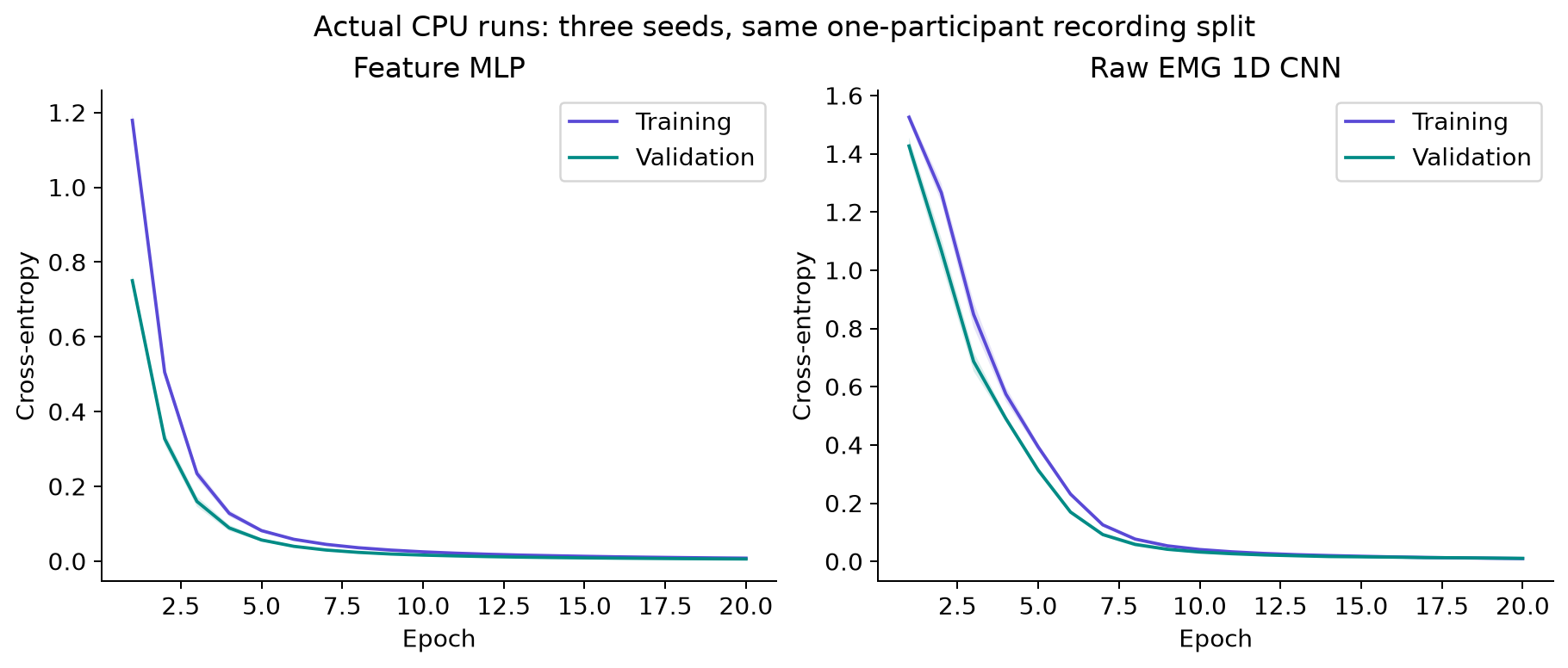
All runs selected epoch twenty, so the best checkpoint reached the training budget rather than an established convergence point. Feature-MLP test balanced accuracies were 99.82%, 100% and 99.64%; raw-CNN scores were 99.64%, 99.64% and 100%. Three seeds measure sensitivity to initialization and minibatch order on this split. They are not three independent datasets.
Ask what the extra flexibility buys
Both models are near the ceiling on these recordings, as are the earlier LDA baselines. This example demonstrates two working training paths; it does not establish a general deep-learning advantage. Compare inference cost, data requirements and failure under changed recording conditions before adopting a more flexible model. Keep class-wise errors and acquisition assumptions visible alongside the training curves.
Try it yourself
Reduce the number of training recording sets while holding validation and test fixed. Compare both networks with the LDA baseline at each training size. Then test whether removing amplitude through per-window normalization changes the errors you expected it to change.
Run the full companion script to regenerate the figures and machine-readable results:
python 06_pytorch.py