Build a reproducible gesture-recognition experiment from the public Myo dataset, preserving recording boundaries from loading through evaluation.
Download the complete runnable series (Python scripts, shared helpers and setup instructions).
Use 64-bit Python 3.11 and LibEMG 2.0.3. Keep the downloaded files together: the walkthrough uses common.py from that bundle. The figures below were generated by these scripts; results describe the stated recordings and split.
Start with a recording, not a classifier
Surface EMG records the superposition of electrical activity from active motor units through a particular electrode arrangement. Its signed waveform fluctuates rapidly; increased activation often increases its amplitude, but electrode placement, contact, force and acquisition hardware also change the observation. A recognizer must learn a reproducible relationship between that observation and a label.
The OneSubjectMyoDataset provides eight channels sampled at 200 Hz, five classes and six recording sets from one person. The stored amplitudes are device counts. We use integer class IDs and the recording metadata: Close, Open, Rest, Extension and Flexion. Two names are reversed in the published wrapper, so trusting the wrapper display names would mislabel the confusion matrix.
python -m pip install -r requirements.txt
    python prepare_data.py myo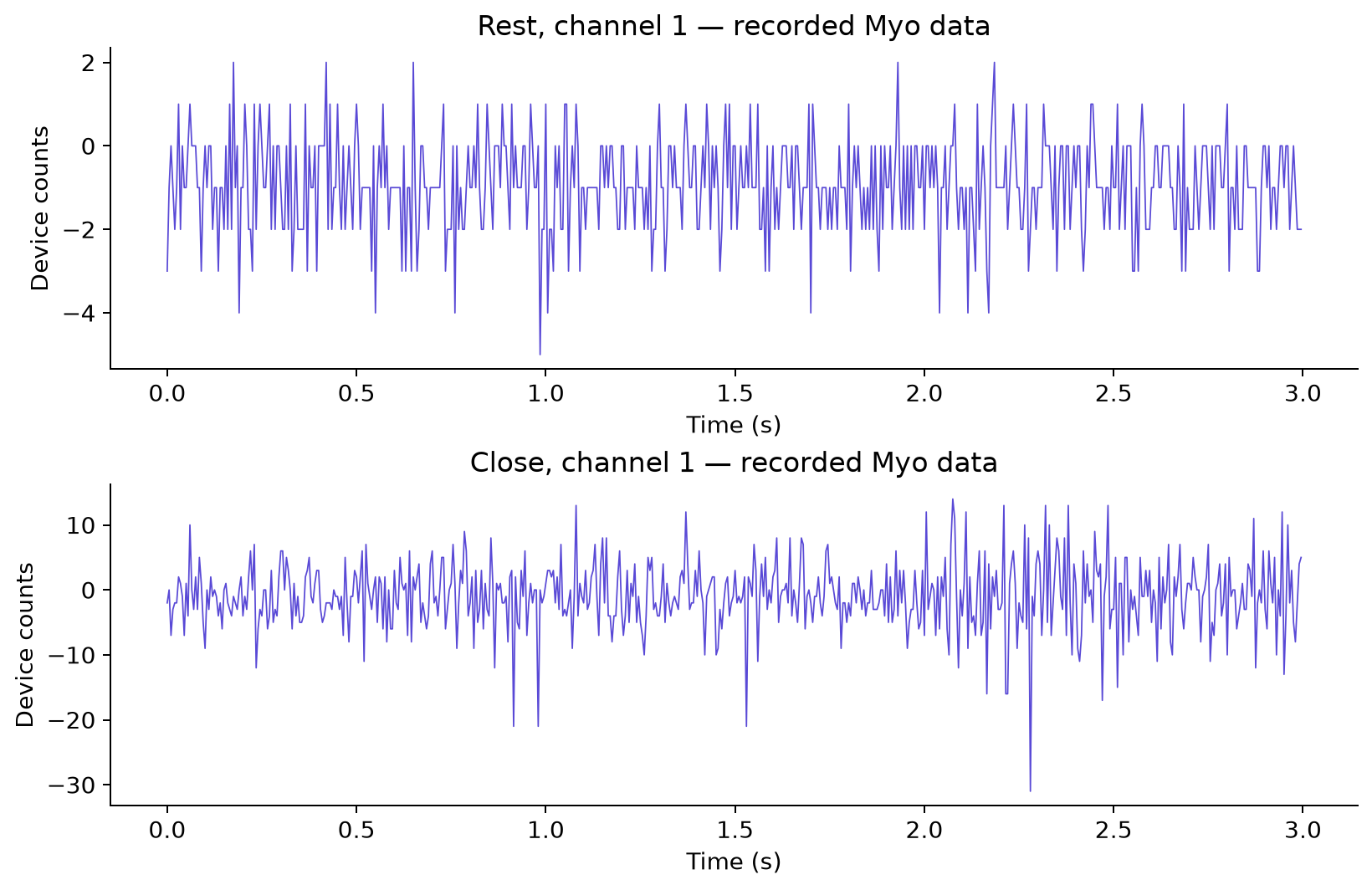
Split whole recordings before overlapping windows
For a recording with \(T\) samples, window length \(N\) and hop \(H\), the window count is \(1+\lfloor(T-N)/H\rfloor\). Here \(N=50\) and \(H=10\): 250 ms of signal and a 50 ms update interval. Adjacent windows share 80% of their samples. Randomly splitting those windows would place almost the same waveform on both sides of evaluation.
The shared loader explicitly assigns zero-based set IDs 0–3 to training, 4 to validation and 5 to testing. These correspond to folders trial_1 through trial_6. LibEMG receives complete recordings before parse_windows is called. Its window arguments are samples, not milliseconds.
from libemg.datasets import OneSubjectMyoDataset
from common import DATA

dataset = OneSubjectMyoDataset(dataset_folder=(DATA / "myo").as_posix() + "/")
recordings = dataset.prepare_data(split=False)
train = recordings.isolate_data("sets", [0, 1, 2, 3], fast=True)
windows, metadata = train.parse_windows(50, 10)
print(windows.shape)  # (2240, 8, 50): windows, channels, samples
import json
import numpy as np
import matplotlib.pyplot as plt
from sklearn.metrics import balanced_accuracy_score, ConfusionMatrixDisplay
from libemg.emg_predictor import EMGClassifier
from common import load_myo, extract, stack, lda, MYO_NAMES, OUT, savefig
dataset, recordings, splits = load_myo()
for name, (windows, metadata) in splits.items():
print(name, windows.shape, 'set IDs:', np.unique(metadata['sets']))The loader returns 2,240 training, 560 validation and 560 test windows. This is a held-recording evaluation within one participant, not an estimate of performance on a new person or after replacing the electrodes. Validation is available for development; the fixed baseline below does not tune its feature pair using the test score.
Compress each channel into two interpretable numbers
Mean absolute value measures average magnitude, \(\mathrm{MAV}=N^{-1}\sum_i |x_i|\). Waveform length measures cumulative sample-to-sample variation, \(\mathrm{WL}=\sum_{i=2}^{N}|x_i-x_{i-1}|\). Eight channels give sixteen inputs. WL reflects both amplitude and temporal variation, so it is not a pure frequency estimate.
common.extract calls LibEMG FeatureExtractor and checks that every returned value is finite. common.stack concatenates families in a fixed order. Feature extraction is deterministic here; the standardization and classifier parameters must be learned from training data only.
Fit a simple LDA through LibEMG
LDA assumes class-conditional Gaussian features with class means \(\mu_k\) and a shared covariance \(\Sigma\). It predicts the class maximizing \(\delta_k(z)=z^T\Sigma^{-1}\mu_k-\tfrac12\mu_k^T\Sigma^{-1}\mu_k+\log\pi_k\). Shared covariance makes this score linear in the feature vector. Correlated inputs can make covariance estimation unstable; automatic shrinkage regularizes that estimate.
common.lda constructs a StandardScaler followed by scikit-learn LDA with solver="lsqr" and shrinkage="auto". The scaler is fitted inside that pipeline. EMGClassifier accepts this estimator and connects it to LibEMG’s training dictionary and prediction interface.
train_w, train_meta = splits['train']
valid_w, valid_meta = splits['validation']
test_w, test_meta = splits['test']
names = ['MAV', 'WL']
x_train = stack(extract(train_w, names), names)
x_valid = stack(extract(valid_w, names), names)
x_test = stack(extract(test_w, names), names)

classifier = EMGClassifier(lda())
classifier.fit({'training_features': x_train,
                'training_labels': train_meta['classes'].astype(int)})
validation_prediction, _ = classifier.run(x_valid)
print('Validation balanced accuracy:', balanced_accuracy_score(
    valid_meta['classes'], validation_prediction))
Read errors, not just an accuracy number
# The feature pair is specified in advance, not chosen by this test score.
prediction, _ = classifier.run(x_test)
result = {'features': names,
          'train_shape': list(train_w.shape), 'validation_shape': list(valid_w.shape),
          'test_shape': list(test_w.shape),
          'validation_balanced_accuracy': float(balanced_accuracy_score(valid_meta['classes'], validation_prediction)),
          'test_balanced_accuracy': float(balanced_accuracy_score(test_meta['classes'], prediction))}
(OUT / '01-results.json').write_text(json.dumps(result, indent=2))
Balanced accuracy averages recall across classes: \(\mathrm{BA}=K^{-1}\sum_k \mathrm{TP}_k/(\mathrm{TP}_k+\mathrm{FN}_k)\). This prevents a frequently sampled class from dominating the score. This run produced 99.82% validation and 98.21% test balanced accuracy. The normalized confusion matrix shows which true classes are confused, rather than only how many predictions are correct.
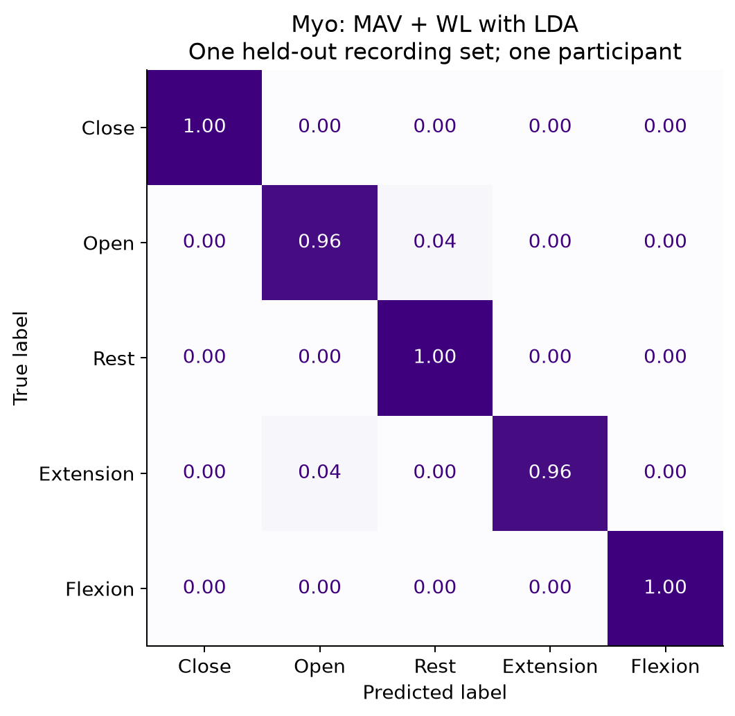
The high score establishes that the loading and learning pipeline works on these recordings. Overlapping windows are correlated observations, so treating all 560 predictions as independent trials would give misleading uncertainty. Later lessons reuse this teaching split; a final research claim would need a fresh evaluation design.
Try it yourself
Change the window length to 100 samples while retaining the recording split. Predict how latency, window count and the stability of MAV change before running it. Compare class-wise errors and report the new duration, not just the new array shape.
Run the full companion script to regenerate the figures and machine-readable results:
python 01_offline.pyLibEMG documentation: offline data and metadata