Connect ten feature families to their equations, compare them with the same LDA classifier, and examine redundancy within and between gestures.
Download the complete runnable series (Python scripts, shared helpers and setup instructions).
Use 64-bit Python 3.11 and LibEMG 2.0.3. Keep the downloaded files together: the walkthrough uses common.py from that bundle. The figures below were generated by these scripts; results describe the stated recordings and split.
Hold the evaluation protocol still
Return to the 200 Hz Myo recordings and the first four training sets from exercise 1. Each development fold holds out one complete set. All feature families use the same windows, labels and scaled shrinkage-LDA pipeline. Changing the classifier for each feature would make it harder to attribute a performance difference to the representation.
Write a channel window as \(x_1,\ldots,x_N\), with \(N=50\), and let \(\bar x\) denote its mean. Most features below produce one number per channel. Four autoregressive coefficients produce four per channel. These are definitions for the exercised LibEMG 2.0.3 implementation; parameter names and normalization matter when comparing another library.
Amplitude and accumulated variation
\(\mathrm{MAV}=N^{-1}\sum_i|x_i|\) captures typical magnitude. \(\mathrm{RMS}=\sqrt{N^{-1}\sum_i x_i^2}\) weights large excursions more strongly. \(\mathrm{VAR}=N^{-1}\sum_i(x_i-\bar x)^2\) removes the window mean and uses population normalization, not \(N-1\). Thus \(\mathrm{RMS}^2=\mathrm{VAR}+\bar x^2\). These features often describe related amplitude information, but a changing offset separates RMS from variance.
\(\mathrm{IAV}=\sum_i|x_i|=N\,\mathrm{MAV}\) is exactly redundant with MAV at fixed length. This implementation does not multiply by a sampling interval. \(\mathrm{WL}=\sum_{i=2}^{N}|x_i-x_{i-1}|\) accumulates variation; \(\mathrm{DASDV}=\sqrt{(N-1)^{-1}\sum_{i=2}^{N}(x_i-x_{i-1})^2}\) emphasizes larger differences. Both respond to amplitude and rate of change. Comparing their values across sampling rates without adjustment is misleading.
Crossings, spectral location and temporal prediction
Zero crossings count strict changes of sign: \(\mathrm{ZC}=\sum_{i=1}^{N-1}\mathbf 1[x_i x_{i+1}<0]\). Samples equal to zero do not create a strict crossing. This version does not expose a ZC amplitude threshold. Slope sign changes use \(\mathrm{SSC}=\sum_{i=2}^{N-1}\mathbf 1[(x_i-x_{i-1})(x_i-x_{i+1})\geq\tau]\). We set SSC_threshold=1.0; the product has squared device-count units. The default zero threshold counts flat products, an important detail for quantized recordings.
Mean frequency is \(\mathrm{MNF}=\sum_k f_k P_k/\sum_k P_k\): the power-weighted spectral centroid. Supply MNF_fs=200, not a differently spelled sampling keyword. Here LibEMG uses the positive half of a padded FFT, without mean removal or Welch averaging, and excludes the Nyquist bin. Padding 50 samples to 64 densifies the frequency grid; it does not improve the underlying approximately 4 Hz resolution of a 250 ms observation.
Order-four autoregression models \(x_t+\sum_{j=1}^{4}a_jx_{t-j}=e_t\). LibEMG returns the four LPC coefficients \(a_j\), with this sign convention. They summarize short-lag predictability and spectral shape. They are neither four amplitude estimates nor a direct measurement of muscle conduction velocity. Flat or degenerate windows can make some feature calculations ill-conditioned; inspect nonfinite outputs instead of silently replacing them.
Extract and verify the identities
import json
import numpy as np
import matplotlib.pyplot as plt
from common import load_myo, extract, stack, held_set_scores, FEATURES, OUT, savefig

_, _, splits = load_myo()
windows, metadata = splits['train']
features = extract(windows)
y, groups = metadata['classes'].astype(int), metadata['sets'].astype(int)
assert np.allclose(features['IAV'], windows.shape[-1] * features['MAV'])
assert np.allclose(features['RMS']**2,
                   features['VAR'] + windows.mean(axis=-1)**2)
The shared helper passes SSC_threshold=1.0, MNF_fs=200 and AR_order=4. The two assertions verify mathematical relationships against actual returned arrays. A feature family with one scalar per channel contributes eight dimensions; AR contributes 32. The classic Hudgins time-domain combination used here, HTD, contains MAV, ZC, SSC and WL, also 32 dimensions.
configurations = {name: [name] for name in FEATURES}
configurations['HTD'] = ['MAV', 'ZC', 'SSC', 'WL']
scores = {name: held_set_scores(stack(features, names), y, groups)
          for name, names in configurations.items()}
result = {name: {'fold_accuracy': values.tolist(), 'mean_accuracy': float(values.mean()),
                 'dimensions': int(stack(features, configurations[name]).shape[1])}
          for name, values in scores.items()}
(OUT/'04-results.json').write_text(json.dumps(result, indent=2))
print(result)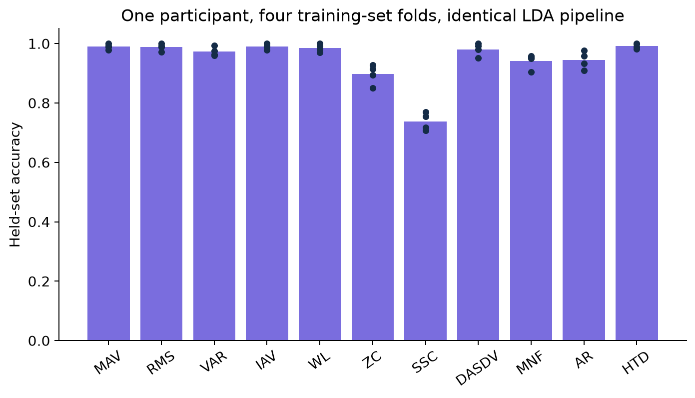
MAV and IAV both averaged 98.97%, WL 98.53%, MNF 94.15%, AR 94.42%, ZC 89.69% and SSC 73.71%. HTD averaged 99.24%. This ranks these representations for this participant and split. It does not establish a universal feature hierarchy: bandwidth, noise, gesture choice and electrode changes can all alter the result.
Separate redundancy from shared class structure
Pearson correlation is \(\rho_{uv}=\mathrm{Cov}(u,v)/(\sigma_u\sigma_v)\). High pooled correlation can arise because two useful features both change between gestures. To examine within-class co-variation, subtract each class mean before calculating the correlation. Neither matrix alone determines whether a feature adds predictive information conditional on the others.
# Inspect channel 1 scalar features; AR has several coefficients and is separate.
scalar_names = [name for name in FEATURES if name != 'AR']
channel = np.column_stack([features[name][:, 0] for name in scalar_names])
centered = channel.copy()
for label in np.unique(y):
    centered[y == label] -= centered[y == label].mean(axis=0)
pooled_correlation = np.corrcoef(channel, rowvar=False)
within_correlation = np.corrcoef(centered, rowvar=False)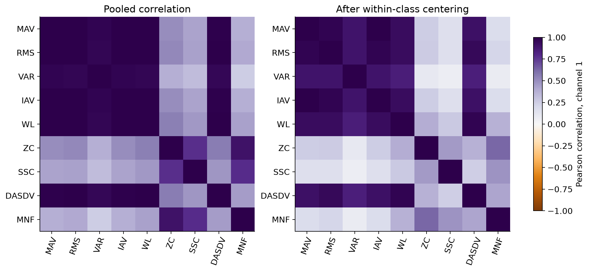
Amplitude-related families share substantial information, while thresholded counts behave differently. The matrices describe one channel and the development data only. Correlation pruning is a useful screening step, but nonlinear dependence and interactions can survive a low pairwise correlation.
Try it yourself
Change SSC_threshold while keeping the grouped folds fixed. Explain its units and count the flat windows. Then compare correlations on each channel separately. Identify one exact redundancy and one merely empirical association before attempting feature selection.
Run the full companion script to regenerate the figures and machine-readable results:
python 04_features.py